Advanced Features

Added Mass

Theoretical Implementation

Added mass is a special multi-directional fluid dynamic phenomenon that most physics software cannot account for well. Modeling difficulties arise because the added mass force is proportional to acceleration. However most time-domain simulations are attempting to use the calculated forces to determine a body’s acceleration, which then determines the velocity and position at the next time step. Solving for acceleration when forces are dependent on acceleration creates an algebraic loop.

The most robust solution is to combine the added mass matrix with the rigid body’s mass and inertia, shown in the manipulation of the governing equation below:

\[\begin{split}M\ddot{X_i} &= \Sigma F(t,\omega) - A\ddot{X_i} \\ (M+A)\ddot{X_i} &= \Sigma F(t,\omega) \\ M_{adjusted}\ddot{X_i} &= \Sigma F(t,\omega)\end{split}\]

where capital \(M\) is the mass matrix, \(A\) is the added mass, and subscript \(i\) represents the timestep being solved for. In this case, the adjusted body mass matrix is defined as the sum of the translational mass (\(m\)), inertia tensor (\(I\)), and the added mass matrix:

\[\begin{split}M_{adjusted} = \begin{bmatrix} m + A_{1,1} & A_{1,2} & A_{1,3} & A_{1,4} & A_{1,5} & A_{1,6} \\ A_{2,1} & m + A_{2,2} & A_{2,3} & A_{2,4} & A_{2,5} & A_{2,6} \\ A_{3,1} & A_{3,2} & m + A_{3,3} & A_{3,4} & A_{3,5} & A_{3,6} \\ A_{4,1} & A_{4,2} & A_{4,3} & I_{1,1} + A_{4,4} & -I_{2,1} + A_{4,5} & -I_{3,1} + A_{4,6} \\ A_{5,1} & A_{5,2} & A_{5,3} & I_{2,1} + A_{5,4} & I_{2,2} + A_{5,5} & -I_{3,2} + A_{5,6} \\ A_{6,1} & A_{6,2} & A_{6,3} & I_{3,1} + A_{6,4} & I_{3,2} + A_{6,5} & I_{3,3} + A_{6,6} \\ \end{bmatrix}\end{split}\]

This formulation is desirable because it removes the acceleration dependence from the right hand side of the governing equation. Without this treatment, the acceleration causes an unsolvable algebraic loop. There are alternative approximations to solve the algebraic loop, but simulation robustness and stability become increasingly difficult.

The core issue with this combined mass formulation is that Simscape Multibody, and most other physics software, do not allow a generic body to have a degree-of-freedom specific mass. For example, a rigid body can’t have one mass for surge motion and another mass for heave motion. Simscape rigid bodies only have one translational mass, a 1x3 moment of inertia matrix, and 1x3 product of inertia matrix.

WEC-Sim’s Implemenation

Due to this limitation, WEC-Sim cannot combine the body mass and added mass on the left-hand side of the equation of motion (as shown above). The algebaric loop can be solved by predicting the acceleration at the current time step, and using that to calculate the added mass force. But this method can cause numerical instabilities. Instead, WEC-Sim decreases the added mass force magnitude by moving some components of added mass into the body mass, while a modified added mass force is calculated with the remainder of the added mass coefficients.

There is a 1-1 mapping between the body’s inertia tensor and rotational added mass coefficients. These added mass coefficients are entirely lumped with the body’s inertia. Additionally, the surge-surge (1,1), sway-sway (2,2), heave-heave (3,3) added mass coefficients correspond to the translational mass of the body, but must be treated identically.

WEC-Sim implements this added mass treatment using both a modified added mass matrix and a modified body mass matrix:

\[\begin{split}M\ddot{X_i} &= \Sigma F(t,\omega) - A\ddot{X_i} \\ (M+dMass)\ddot{X_i} &= \Sigma F(t,\omega) - (A-dMass)\ddot{X_i} \\ M_{adjusted}\ddot{X_i} &= \Sigma F(t,\omega) - A_{adjusted}\ddot{X_i} \\\end{split}\]

where \(dMass\) is the change in added mass and defined as:

\[\begin{split}dMass &= \begin{bmatrix} \alpha Y & 0 & 0 & 0 & 0 & 0 \\ 0 & \alpha Y & 0 & 0 & 0 & 0 \\ 0 & 0 & \alpha Y & 0 & 0 & 0 \\ 0 & 0 & 0 & A{4,4} & -A{5,4} & -A{6,4} \\ 0 & 0 & 0 & A{5,4} & A{5,5} & -A{6,5} \\ 0 & 0 & 0 & A{6,4} & A{6,5} & A{6,6} \\ \end{bmatrix} \\ Y &= (A_{1,1} + A_{2,2} + A_{3,3}) \\ \alpha &= body(iBod).adjMassFactor\end{split}\]

The resultant definition of the body mass matrix and added mass matrix are then:

\[\begin{split}M &= \begin{bmatrix} m + \alpha Y & 0 & 0 & 0 & 0 & 0 \\ 0 & m + \alpha Y & 0 & 0 & 0 & 0 \\ 0 & 0 & m + \alpha Y & 0 & 0 & 0 \\ 0 & 0 & 0 & I_{4,4} + A_{4,4} & -(I_{5,4} + A_{5,4}) & -(I_{6,4} + A_{6,4}) \\ 0 & 0 & 0 & I_{5,4} + A_{5,4} & I_{5,5} + A_{5,5} & -(I_{6,5} + A_{6,5}) \\ 0 & 0 & 0 & I_{6,4} + A_{6,4} & I_{6,5} + A_{6,5} & I_{6,6} + A_{6,6} \\ \end{bmatrix} \\ A_{adjusted} &= \begin{bmatrix} A_{1,1} - \alpha Y & A_{1,2} & A_{1,3} & A_{1,4} & A_{1,5} & A_{1,6} \\ A_{2,1} & A_{2,2} - \alpha Y & A_{2,3} & A_{2,4} & A_{2,5} & A_{2,6} \\ A_{3,1} & A_{3,2} & A_{3,3} - \alpha Y & A_{3,4} & A_{3,5} & A_{3,6} \\ A_{4,1} & A_{4,2} & A_{4,3} & 0 & A_{4,5} + A_{5,4} & A_{4,6} + A_{6,4} \\ A_{5,1} & A_{5,2} & A_{5,3} & 0 & 0 & A_{5,6} + A_{6,5} \\ A_{6,1} & A_{6,2} & A_{6,3} & 0 & 0 & 0 \\ \end{bmatrix}\end{split}\]

Note

We should see that \(A_{4,5} + A_{5,4} = A_{4,6} + A_{6,4} = A_{5,6} + A_{6,5} = 0\), but there may be numerical differences in the added mass coefficients which are preserved.

Though the components of added mass and body mass are manipulated in WEC-Sim, the total system is unchanged. This manipulation does not affect the governing equations of motion, only the implementation.

The fraction of translational added mass that is moved into the body mass is determined by body(iBod).adjMassFactor, whose default value is \(2.0\). Advanced users may change this weighting factor in the wecSimInuptFile to create the most robust simulation possible. To see its effects, set body(iB).adjMassFactor = 0 and see if simulations become unstable.

This manipulation does not move all added mass components. WEC-Sim still contains an algebraic loop due to the acceleration dependence of the remaining added mass force from \(A_{adjusted}\), and components of the Morison Element force. WEC-Sim solves the algebraic loop using a Simulink Transport Delay with a very small time delay (1e-8). This blocks extrapolates the previous acceleration by 1e-8 seconds, which results in a known acceleration for the added mass force. The small extraplation solves the algebraic loop but prevents large errors that arise when extrapolating the acceleration over an entire time step. This will convert the algebraic loop equation of motion to a solvable one:

\[\begin{split}M_{adjusted}\ddot{X_i} &= \Sigma F(t,\omega) - A_{adjusted}\ddot{X}_{i - (1 + 10^{-8}/dt)} \\\end{split}\]

Working with the Added Mass Implementation

WEC-Sim’s added mass implementation should not affect a user’s modeling workflow. WEC-Sim handles the manipulation and restoration of the mass and forces in the bodyClass functions adjustMassMatrix() called by initializeWecSim and restoreMassMatrix, storeForceAddedMass called by postProcessWecSim. However viewing body.mass, body.inertia, body,inertiaProducts, body.hydroForce.fAddedMass between calls to initializeWecSim and postProcessWecSim will not show the input file definitions. Users can get the manipulated mass matrix, added mass coefficients, added mass force and total force from body.hydroForce.storage after the simulation. However, in the rare case that a user wants to manipulate the added mass force during a simulation, the change in mass, \(dMass\) above, must be taken into account. Refer to how body.calculateForceAddedMass() calculates the entire added mass force in WEC-Sim post-processing.

Note

If applying the method in body.calculateForceAddedMass() during the simulation, the negative of dMass must be taken: \(dMass = -dMass\). This must be accounted for because the definitions of mass, inertia, etc and their stored values are flipped between simulation and post-processing.

Note

Depending on the wave formulation used, \(A\) can either be a function of wave frequency \(A(\omega)\), or equal to the added mass at infinite wave frequency \(A_{\infty}\)

Morison Element

As a reminder from the WEC-Sim Theory Manual, the Morison force equation assumes that the fluid forces in an oscillating flow on a structure of slender cylinders or other similar geometries arise partly from pressure effects from potential flow and partly from viscous effects. A slender cylinder implies that the diameter, \(D\), is small relative to the wave length, \(\lambda\), which is generally satisfied when \(D/\lambda<0.1-0.2\). If this condition is not met, wave diffraction effects must be taken into account. Assuming that the geometries are slender, the resulting force can be approximated by a modified Morison formulation for each element on the body.

Fixed Body

For a fixed body in an oscillating flow the force imposed by the fluid is given by:

(1)\[\vec{F}_{ME} = \underbrace{\rho \forall C_{m} \dot{\vec{u}}}_{\text{Inertia}} + \underbrace{\frac{1}{2} \rho A C_{D} \vec{u} | \vec{u} |}_{Drag}\]

where \(\vec{F}_{ME}\) is the Morison element hydrodynamic force, \(\rho\) is the fluid density, \(\forall\) is the displaced volume, \(C_{m}\) is the inertia coefficient, \(A\) is the reference area, \(C_{D}\) is the drag coefficient, and \(u\) is the fluid velocity. The inertia coefficient is defined as:

(2)\[C_{m} = 1 + C_{a}\]

where \(C_{a}\) is the added mass coefficient. The inertia term is the sum of the Froude- Krylov Force, \(\rho \forall \dot{u}\), and the hydrodynamic mass force, \(\rho C_{a} \forall \dot{u}\). The inertia and drag coefficients are generally obtained experimentally and have been found to be a function of the Reynolds (Re) and Kulegan Carpenter (KC) numbers

(3)\[\text{Re} = \frac{U_{m}D}{\nu}~~\&~~ \text{KC} = \frac{U_{m}T}{D}~~\]

where \(U_{m}\) is the maximum fluid velocity, and \(\nu\) is the kinematic viscosity of the fluid, and \(T\) is the period of oscillation. Generally when KC is small then \(\vec{F}\) is dominated by the inertia term when the drag term dominates at high KC numbers. If the fluid velocity is sinusoidal then \(u\) is given by:

(4)\[u(t) = U_{m} \sin \left( \sigma t \right)~~\]

where \(\sigma = 2\pi/T\). This can be taking further by considering the body is being is impinged upon by regular waves of the form:

(5)\[\begin{split}\eta(x,t) & = A \cos \left( \sigma t - k \left[ x \cos \theta + y \sin \theta\right] \right) = \Re \left\lbrace -\frac{1}{g}\frac{\partial \phi_{I}}{\partial t} \bigg|_{z=0} \right\rbrace~~, \\ \phi_{I}(x,z,t) & = \Re \left\lbrace \frac{Ag}{\sigma} \frac{\cosh \left(k (z+h) \right)}{\cosh \left( kh \right)} i e^{i(\sigma t-k\left[ x \cos \theta + y \sin \theta\right])} \right\rbrace~~, \\ \sigma^{2} & = gk\tanh\left(kh\right)\end{split}\]

where \(\eta\) is the wave elevation, \(\phi_{I}\) is the incident wave potential, \(A\) is the wave amplitude, \(k\) is the wave number (defined as \(k=\frac{2\pi}{\lambda}\) where \(\lambda\) is the wave length), \(g\) is gravitational acceleration, \(h\) is the water depth, \(z\) is the vertical position in the water column, \(\theta\) is the wave heading. The fluid velocity can then be obtained by taking the graident of Eqn. (5) :

(6)\[\begin{split}u (x,z,t) & = \Re \left\lbrace \frac{\partial \phi_{I}}{\partial x} \right\rbrace = \frac{Agk}{\sigma} \frac{\cosh \left( k (z+h)\right)}{\cosh \left( kh \right)} \cos \left( \sigma t - k x \right) \cos\left(\theta\right)~~,\\ v (x,z,t) & = \Re \left\lbrace \frac{\partial \phi_{I}}{\partial y} \right\rbrace = \frac{Agk}{\sigma} \frac{\cosh \left( k (z+h)\right)}{\cosh \left( kh \right)} \cos \left( \sigma t - k x \right)\sin\left(\theta\right)~~,\\ w (x,z,t) & = \Re \left\lbrace \frac{\partial \phi_{I}}{\partial z} \right\rbrace = -\frac{Agk}{\sigma} \frac{\sinh \left( k (z+h)\right)}{\cosh \left( kh \right)} \sin \left( \sigma t - k x \right)~~,\end{split}\]

The acceleration of the fluid particles will then be obtained by taking the time derivative of Eqn. (6) :

(7)\[\begin{split}\dot{u} (x,z,t) & = \frac{\partial u}{\partial t} = -Agk \frac{\cosh \left( k (z+h)\right)}{\cosh \left( kh \right)} \sin \left( \sigma t - k x \right) \cos\left(\theta\right)~~,\\ \dot{v} (x,z,t) & = \frac{\partial v}{\partial t} = -Agk \frac{\cosh \left( k (z+h)\right)}{\cosh \left( kh \right)} \sin \left( \sigma t - k x \right) \sin\left(\theta\right)~~,\\ \dot{w} (x,z,t) & = \frac{\partial w}{\partial t} = -Agk \frac{\sinh \left( k (z+h)\right)}{\cosh \left( kh \right)} \cos \left( \sigma t - k x \right)~~,\end{split}\]

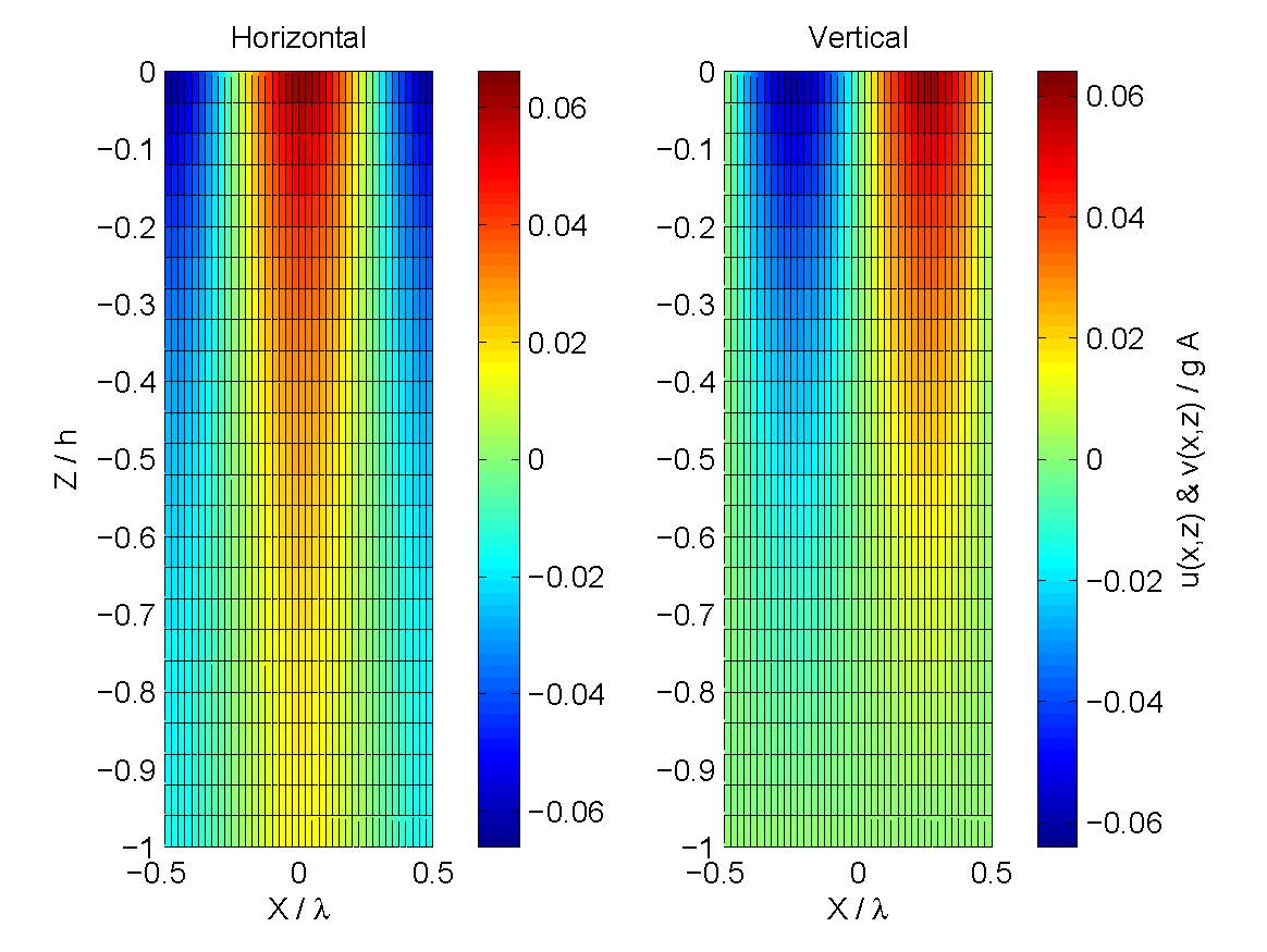
Horizontal and vertical orbital velocity magnitude for a wave period of 10 s and water depth of 50 m with a wave heading of 0 rads.

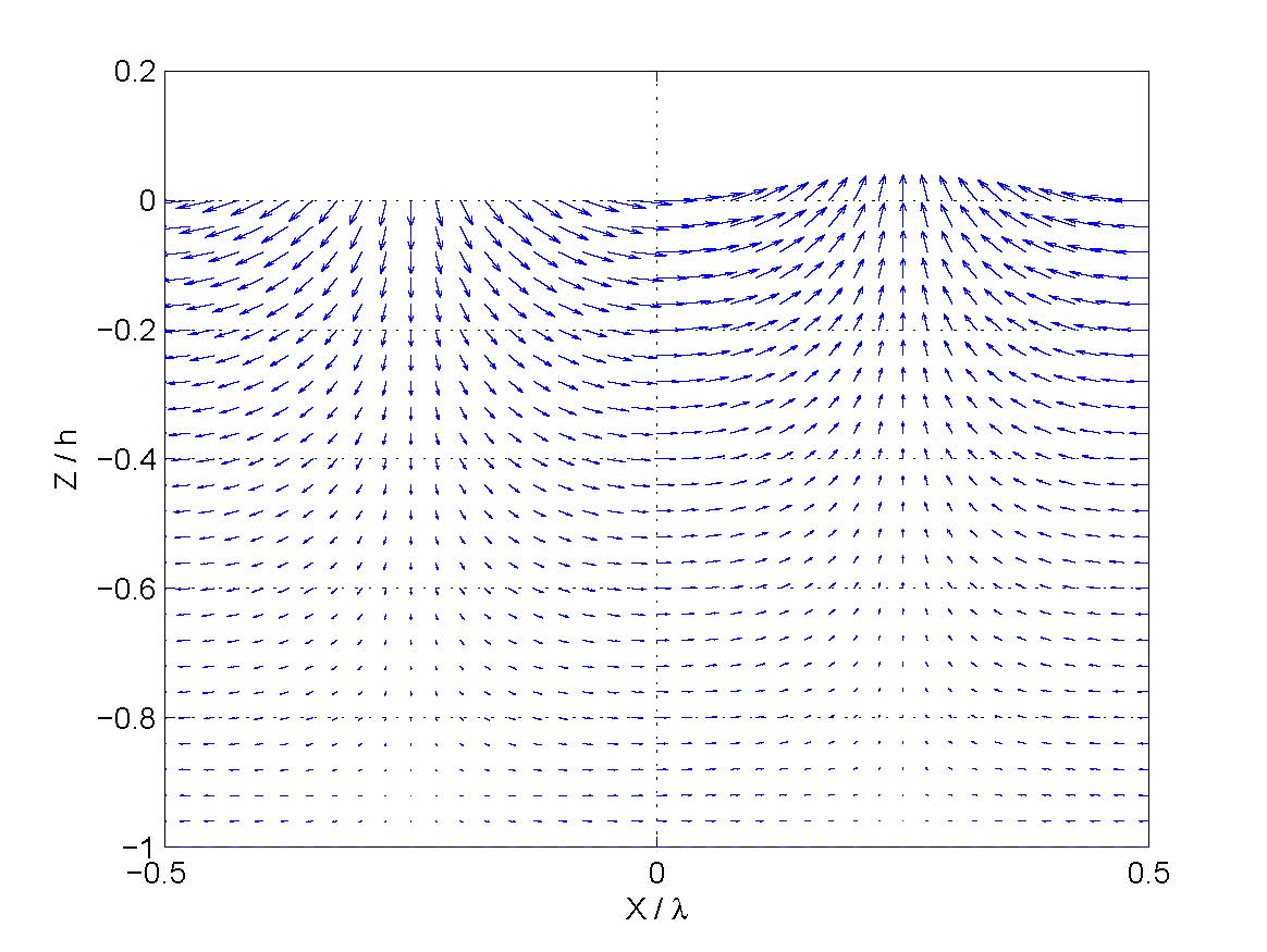
Orbital velocity magnitude vectors for a wave period of 10 s and water depth of 50 m with a wave heading of 0 rads.

Moving Body

If the body is allowed to move in an oscillating flow then Eqn. (1) must be adjusted as follows:

(8)\[\vec{F}_{ME} = \rho \forall \dot{\vec{u}} + \rho \forall C_{a} \left( \dot{\vec{u}} - \dot{\vec{U}} \right) + \frac{1}{2}\rho C_{D} A \left( \vec{u} - \vec{U} \right) \left| \vec{u} - \vec{U} \right|~~\]

where \(U\) is the body velocity. In the calculations performed by WEC-Sim, it is assumed that the body does not alter the wave field and the fluid velocity and acceleration can be calculated from the incident wave potential as from Eqn. (6) and (7).

Review of Rigid Body Dynamics

A rigid body is an idealization of a solid body in which deformation is neglected. In other words, the distance between any two given points of a rigid body remains constant in time regardless of external forces exerted on it. The position of the whole body is represented by its linear position together with its angular position with a global fixed reference frame. WEC-Sim calculates the position, velocity, and acceleration of the rigid body about its center of gravity; however, the placement of each morrison element will have a different local velocity that affects the fluid force. The relative velocity between point A and point B on a rigid body is given by:

(9)\[\vec{U}_{A} = \vec{U}_{B} + \omega \times r_{BA}~~\]

where \(\omega\) is the angular velocity of the body and \(\times\) denotes the cross product. Taking the time derivative of Eqn. (9) provides the relative acceleration:

(10)\[\vec{\dot{U}}_{A} = \vec{\dot{U}}_{B} + \omega \times \omega \times r_{BA} + \dot{\omega} \times r_{BA}~~\]

WEC-Sim Implementations

As discussed in the WEC-Sim user manual, there are two options to model a Morison element(s) and will be described here in greater detail so potential developers can modify the code to suit their modeling needs.

Option 1

In the first Morison element implementation option, the acceleration and velocity of the fluid flow are estimated at the Morison point of application, which can include both wave and current contributions, and then subtracts the body acceleration and velocity for the individual translational degrees of freedom (x-, y-, and z-components). The fluid flow properties are then used to calculate the Morison element force, indepenently for each degree of freedom, as shown by the following expressions:

(11)\[\begin{split}F_{ME,x} & = \rho \forall \dot{u}_{x} + \rho \forall C_{a,x} \left( \dot{u}_{x} - \dot{U}_{x} \right) + \frac{1}{2}\rho C_{D,x} A_{x} \left( u_{x} - U_{x} \right) \left| u_{x} - U_{x} \right|~~, \\ F_{ME,y} & = \rho \forall \dot{u}_{y} + \rho \forall C_{a,y} \left( \dot{u}_{y} - \dot{U}_{y} \right) + \frac{1}{2}\rho C_{D,y} A_{y} \left( u_{y} - U_{y} \right) \left| u_{y} - U_{y} \right|~~, \\ F_{ME,z} & = \rho \forall \dot{u}_{z} + \rho \forall C_{a,z} \left( \dot{u}_{z} - \dot{U}_{z} \right) + \frac{1}{2}\rho C_{D,z} A_{z} \left( u_{z} - U_{z} \right) \left| u_{z} - U_{z} \right|~~, \\ \vec{M} & = \vec{r} \times \vec{F} = \left[ r_{g,x}, r_{g,y}, r_{g,z} \right] \times \left[ F_{x}, F_{y}, F_{z} \right]\end{split}\]

where \(r_{g}\) is the lever arm from the center of gravity of the body to the Morison element point of application. Option 1 provides the most flexibility in setting independent Morison element properties for the x-, y-, and z-directions; however, a limitation arises that the fluid flow magnitude does not consider the other fluid flow components. Depending on the simulation enviroment this approach can provide the same theoretical results as taking the magnitude of the x-, y-, and z-components of the fluid flow, but is case dependent. A comparison between the outputs of Option 1 and Option 2 can be found later in the Developer Manual Morison Element documentation.

Option 2

The WEC-Sim Option 1 implementation solves for the of the Morison element force from the individual x-, y-, and z-components of the relative flow velocity and acceleration; however, this results in incorrect outputs at certain orientations of the flow and Morison Element. As opposed to solving for the x-, y-, and z-components of the Morison element force, the force can be calculated relative to the magnitude of the flow and distributed among its unit vector direction. Therefore the approach used in Option 2 is to decompose the fluid and body velocity and acceleration into tangential and normal components of the Morison element, as depicted in Figure Schematic of the water flow vector decomposition reletive to the Morison Element orientation.

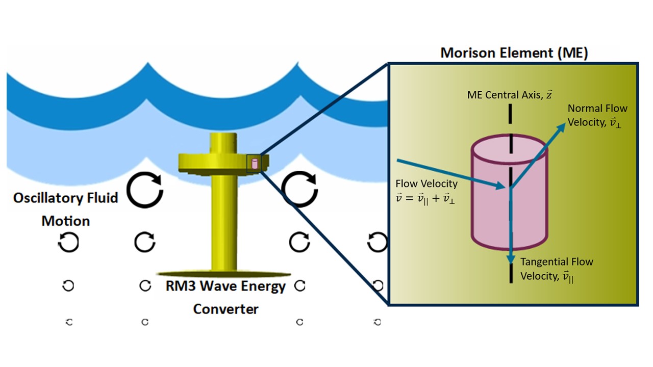
Schematic of the water flow vector decomposition reletive to the Morison Element orientation.

In mathematics, for a given vector at a point on a surface, the vector can be uniquely decomposed into the sum of its tangential and normal components. The tangential component of the vector, \(v_{\parallel}\), is parallel to the surface while the normal component of the vectors, \(v_{\perp}\), is perpendicular to the surface which is used in relation to the central axis to the Morison element. The WEC-Sim input file was altered to consider a tangential and normal component for the drag coefficient [\(C_{d\perp}\) , \(C_{d\parallel}\)] , added mass coefficient [\(C_{a\perp}\) , \(C_{a\parallel}\)], characteristic area [\(A_{\perp}\) , \(A_{\parallel}\)], and the central axis vector of the ME = [ \(\vec{z} = `:math:`z_{x}\) , \(z_{y}\) , \(z_{z}\) ].

A general vector, \(\vec{k}\), can be decomposed into the normal component as a projection of vector k on to the central axis z as follows:

(12)\[\vec{k}_{\parallel} = \frac{\vec{z} \cdot \vec{k}}{ || \vec{z} || } \frac{ \vec{z} }{ || \vec{z} || }\]

As the vector \(\vec{k}\) is uniquely decomposed into the sum of its tangential and normal components, the normal component can be defined as the difference between the vector \(\vec{k}\) and its tangential component as follows:

(13)\[\vec{k}_{\perp} = \vec{k} - \vec{k}_{\parallel}\]

Using this vector multiplication, the tangential and normal components of the fluid flow can be obtained as follows:

(14)\[\begin{split}\vec{u}_{\parallel} = \frac{\vec{z} \cdot \vec{u}}{ || \vec{z} || } \frac{ \vec{z} }{ || \vec{z} || } \\ \vec{u}_{\perp} = \vec{u}-\vec{u}_{\perp}\end{split}\]

The Morison element force equation for a moving body relative to the fluid flow is modified to include the following decomposition of force components and consider the magnitude of the flow:

(15)\[\begin{split}\vec{F}_{ME} = \rho C_{M,\parallel} \forall \left( \dot{\vec{u}}_{\parallel} - \dot{\vec{U}}_{\parallel} \right) + \frac{1}{2}\rho C_{d,\parallel} \left( \vec{v}_{\parallel} - \vec{U}_{\parallel} \right) \lvert \vec{v}_{\parallel} - \vec{U}_{\parallel} \rvert + \\ \rho C_{M,\perp} \forall \left( \dot{\vec{u}}_{\perp} - \dot{\vec{U}}_{\perp} \right) + \frac{1}{2}\rho C_{d,\perp} \left( \vec{v}_{\perp} - \vec{U}_{\perp} \right) \lvert \vec{v}_{\perp} - \vec{U}_{\perp} \rvert\end{split}\]

Comparison of Performance Between Option 1 and Option 2

A simple test case, which defines a Morison element as vertical and stationary relative to horizontal fluid flow, was built to compare the Morison element force calculation between Option 1 and Option 2 within WEC-Sim. Theoretically, the magnitude of the Morison element force should remain constant as the orientation of the flow direction is rotated in the X-Y plane. The MF was calculated as the orientation of the flow was rotated about the z-axis from 1 to 360 degrees where the central axis of the ME is parallel wtih the z-axis. The remaining WEC-Sim input values for the simulation can be found in the following table.

Variable Type	Variable Symbol	WEC-Sim Input Values
ME Central Axis	\(\vec{z}\)	[0, 0 , 1]
Fluid flow velocity	\(\vec{U}\)	[-1, 0, 0] \(m/s\)
Fluid flow acceleration	\(\vec{\dot{U}}\)	[-1, 0, 0] \(m/s^{2}\)
Drag Coefficient	\(C_{D}\)	[1, 1, 0]
Mass Coefficient	\(C_{a}\)	[1, 1, 0]
Area	\(A\)	[1, 1, 0]
Density	\(\rho\)	1000 \(kg/m^{3}\)
Displaced Volume	\(\forall\)	0.10 \(m^{3}\)

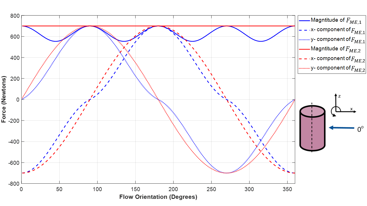
Graphical representation of the comparison between ME Option 1 and Option 2 within WEC-Sim.

\(F_{ME,1}\) and \(F_{ME,2}\) is the Morison element force output from Option 1 and Option 2 within WEC-Sim, respectively. Shown in the above figure, in Option 1 there is an oscillation in Morison element magnitude with flow direction while Option 2 demonstrates a constant force magnitude at any flow direction. The reason behind this performance is that Option 1 solves for the MF individually using the individual the x-, y-, and z- components of the flow while Option 2 calculates the force relative to the flow magnitude and distributed among the normal and tangential unit vectors of the flow.

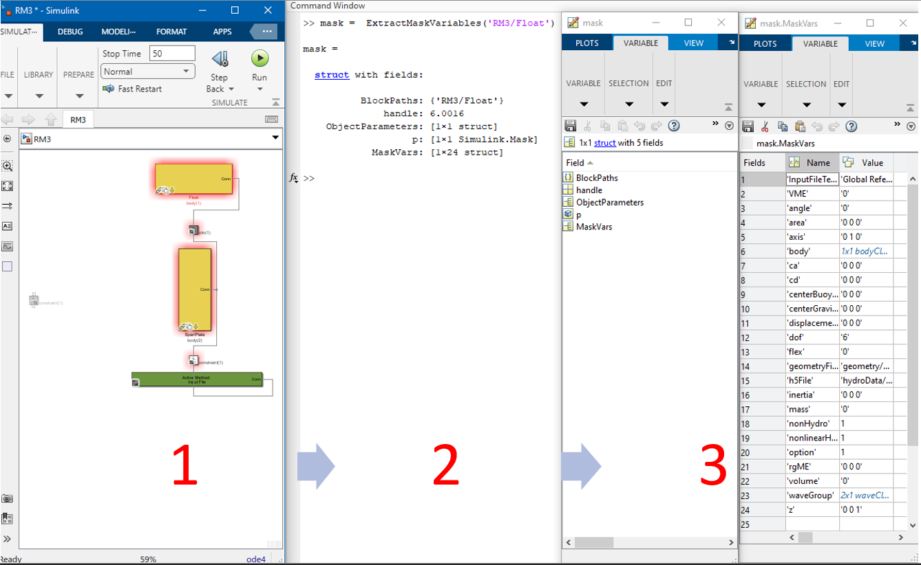
Extract Mask Variables

The Simulink variable workspace is inaccesible in the MATLAB workspace by default. Simulink variables can be imported to the MATLAB workspace using the block handle of the Simulink block being probed. The block parameters can be used by developers to programmatically set block parameters by being able to access the unique tags that Simulink uses for a particular block parameter. This is also useful for the code initialization of Simulink mask blocks. The function ExtractMaskVariables() located in sourcefunctionssimulinkmask, can be used to extract the block parameters in following steps,

• Open the pertinent Simulink model,

• Run the function with the address of the block being probed as the argument,

• Explore the mask data structure in the MATLAB workspace.