Examples ¶

This page includes a number of examples demonstrating the usage of the WDRT. In addtion to code snippets included here, these examples are outlined in the $WDRT_SOURCE/examples directory. Each toolbox module has at least one example/tutorial. The table of contents below gives an outline of the available tutorials.

Contents

Examples

Environmental characterization ¶

The WDRT includes a package for creating environmental contours of extreme sea states using a principle components analysis (PCA) methodology with additional improvements for characterizing the joint probability distribution of sea state variables of interest. Environmental contours describing extreme sea states can be used for numerical or physical model simulations analyzing the design-response of WECs. These environmental contours, characterized by combinations of significant wave height ($H_s$) and either energy period ($T_e$) or peak period ($T_p$), provide inputs that are associated with a certain reliability interval. These reliability levels are needed to drive both contour and full sea state style long-term extreme response analyses.

For this example ($WDRT_SOURCE/examples/example_envSampling.py), we will consider NDBC buoy 46022.

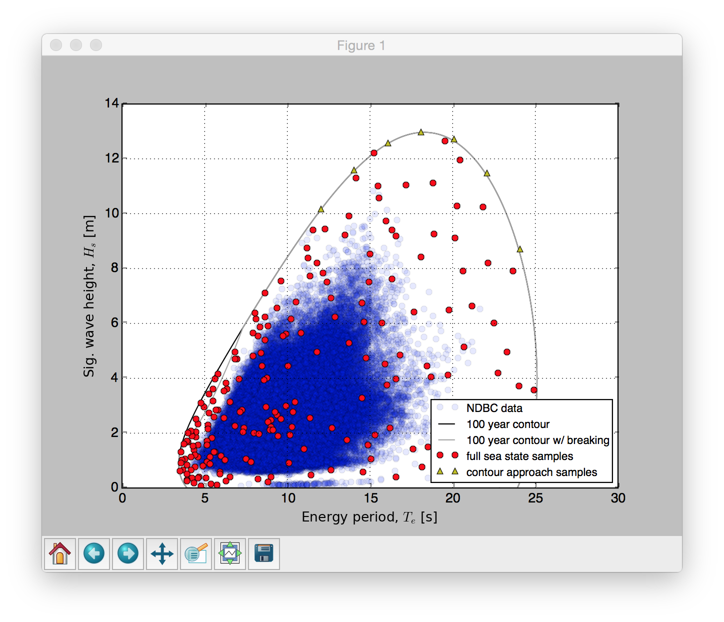
Environmental characterization with NDBC data, 100-year return contour, full sea state samples and contour samples.¶

Short-term extreme response analysis ¶

A short term extreme distribution is the answer to “If a device is in sea-state X for Y amount of time, what will be the largest Z observed?”, where X is the environmental condition, Y the short-term period, and Z the response parameter of interest (e.g. the mooring load, bending moment). The short-term extreme response module provides five different methods for obtaining this distribution based on observations of the quantity of interest “Z” at the desired sea-state “X”. These methods are described in detail in Michelen and Coe 2015.

In this example the Weibull tail-fit method is used. The process of obtaining the sort-term extreme distribution using the Weibull tail-fit method is as follows:

1. Identify the peaks from a time-series of any length of the response “Z” of the WEC in the sea-state of interest “X”. Some minimum time length is required to achieve convergence.

Order the peaks in ascending order and approximate the empirical peak distribution as:

\[F^{\prime}(x_i) = \frac{i}{N+1}\]

where $x_i$ is the $i^{\textrm{th}}$-ordered peak.

Fit Weibull distributions to seven subsets of the points ($x_i$, $F^{\prime}(x_i)$) corresponding to $F^{\prime}(x_i) > \left(0.95, 0.90, 0.85, 0.80, 0.75, 0.70, 0.65 \right)$.

The distribution of the global peaks is then approximated as a Weibull distribution with parameters equal to the average of the parameters of the seven fitted Weibull distributions.

The short term extreme distribution ($F_e(x)$) is then obtained from the peaks distribution ($F_p(x)$) as

\[F_e(x) = F_p(x)^q\]

where $q$ is the number of expected peaks in the short-term period.

In this example we start with a time-series of the quantity of interest at the desired sea-state. The global peaks are then identified.

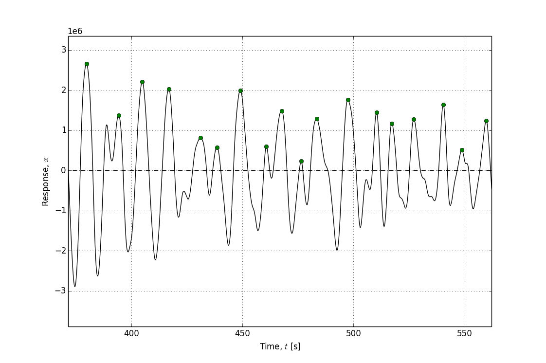
The desired short-term period is 1 hour. The 1-hour extreme distribution is estimated using the Weibull tail fit as described above.

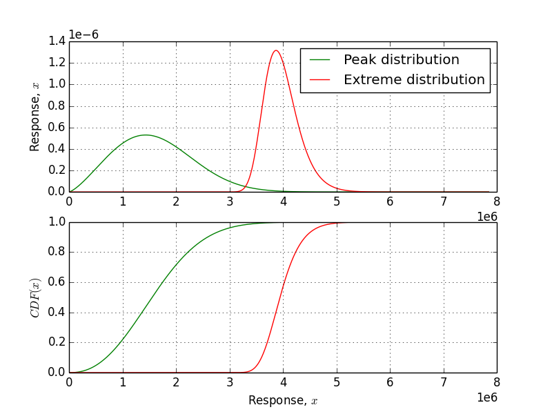
The goodness of fit plots are shown as a visual check. They show the quality of the agreement between the global peaks and the resulting Weibull tail fit.

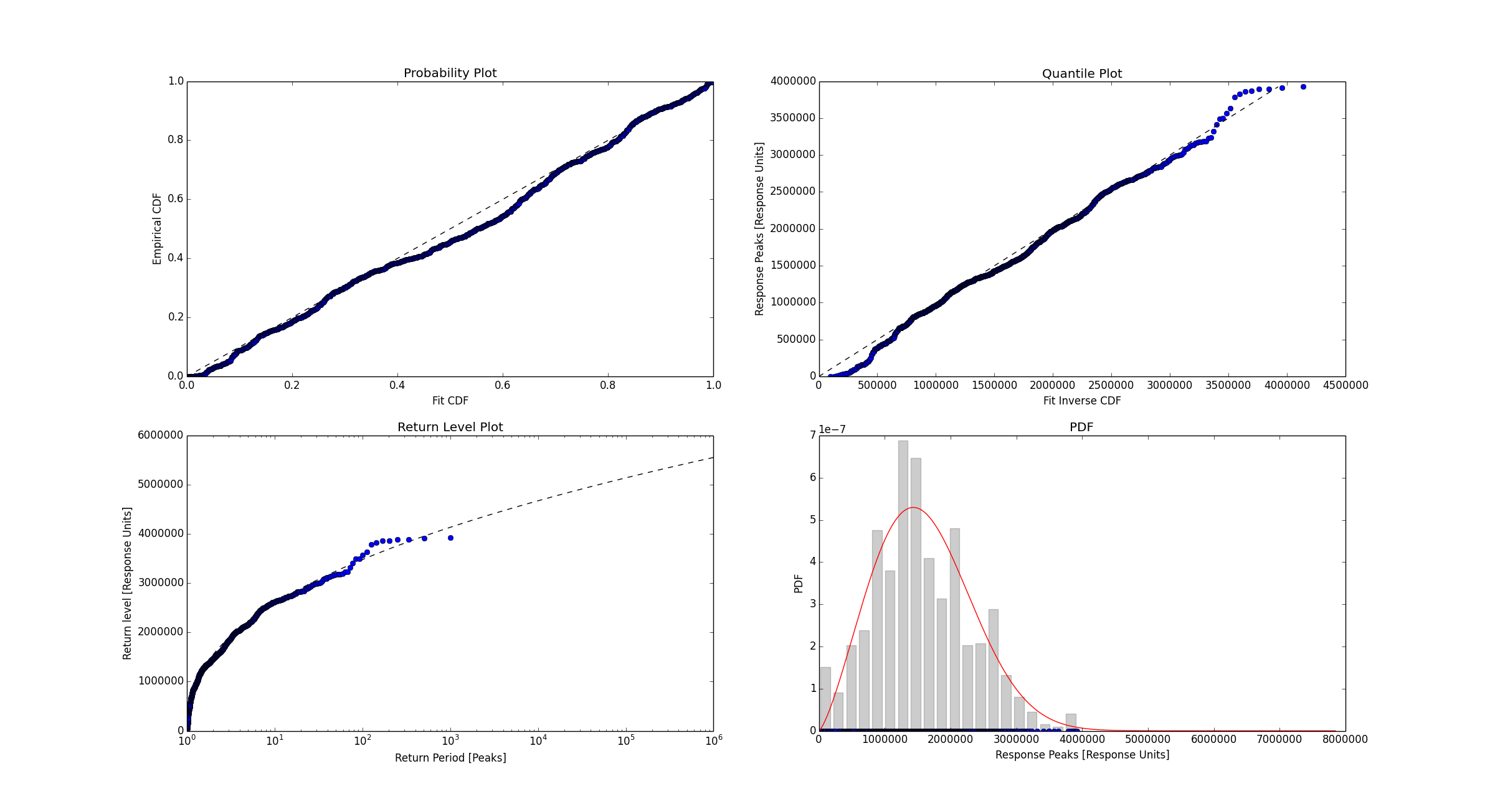
This example is shown below and can found in $WDRT_SOURCE/examples/example_shortTermExtreme.py.

Long-term extreme response analysis ¶

The long-term extreme response represents the design response for some specific deployment location and time-span. Two major classes of approaches are implemented in the WDRT: a Contour approach and a Full sea-sate approach.

Contour approach ¶

In the contour approach, simulations are run along the desired extreme wave contour (e.g. 25-year contour). The condition producing the largest response is used to define the extreme response distribution for the device via a short-term extreme process. To obtain a single design response value for this method, one should select a percentile from that extreme response distribution based on some prior knowledge of system behavior. Typical percentiles used for marine structures range from 75 to 99%.

The following steps demonstrate the execution of a contour approach to long-term extreme response analysis. These steps are also summarized in $WDRT_SOURCE/examples/example_contourApproach.py.

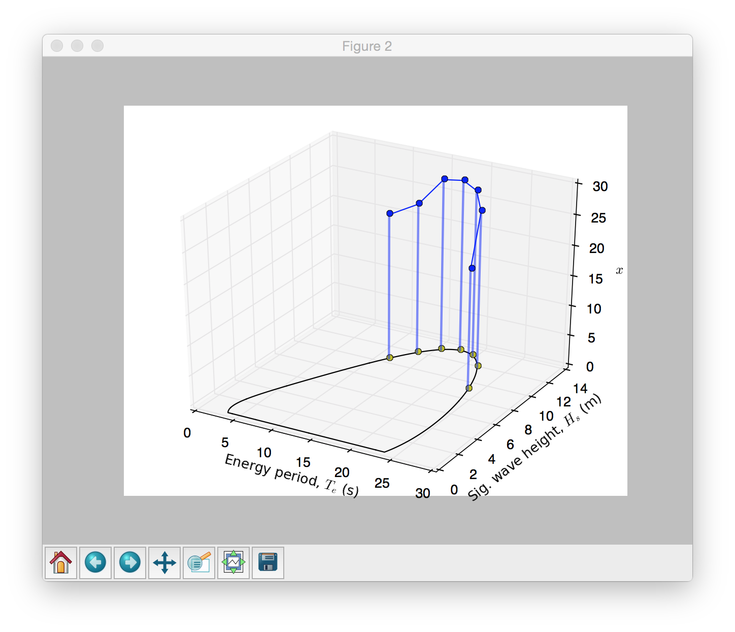
Environmental characterization with NDBC data, 100-year return contour, full sea state samples and contour samples.¶

1. Establish environmental data and sample sea stats ¶

Following the Environmental characterization example, a the environmental conditions at a site can be characterized then sampled to provide a set of sea states for modeling analysis. For this example, we will work with the data produced in the Environmental characterization example.

2. Model device response ¶

Obtain predictions for your device response at each of the selected sea states. This step can be accomplished via any model considered appropriate. Low and mid-fidelity numerical models (e.g. Cummins equation) are often used. However, experimental testing could be used as well. Whatever the approach, the process must supply sufficient time histories of the relevant responses at each of the selected sea states. For this example, we will simply load data that was previously produced with a simple Cummins equation model.

3. Short term extreme statistics ¶

The extreme response for each sea state can be defined as a percentile, $\alpha$, in the extreme response distributions. The percentile chosen here should ideally be based on some experience with similar systems. Typical values for $\alpha$ used for marine structures range from 75 to 99%. This approach has less variability than simply picking the maximum QOI observed in each sea state. Here, we apply a Weibull tail fitting method as discussed further in the Short-term extreme response analysis example.

4. Determine design load condition(s)¶

For the quantity of interest (QOI), find the sea state that represents the design load condition; this will be the design load condition (DLC) for that (QOI). The DLC is defined as the scenario that gives the largest response. To define the DLC by statistically-supported process, it is best to use a short-term extreme response analysis process to examine the QOI in each of the considered sea states.

Full sea-sate approach ¶

In the full sea state approach, simulations are run at a sampling of sea states within an envelop defined by the environmental characterization process. Based on the device response and relative occurrence likelihood for each sea state, an extreme distribution is constructed. The full sea-state approach is more rigorous than the contour approach, but also requires more modelling to implement. This distribution gives a richer picture of the design response and can, for example, be used to study how the design response varies with return period.

The following example is also located at $WDRT_SOURCE/examples/example_longTermFullSeaState.py.

1. Establish environmental data and sample sea states ¶

Following the Environmental characterization example, the environmental conditions at a site can be characterized then sampled to provide a set of sea states for modelling analysis. For this example, we will work with the data produced in the Environmental characterization example.

2. Model device response ¶

Obtain predictions for your device response at each of the selected sea states. This step can be accomplished via any model considered appropriate. Low and mid-fidelity numerical models (e.g. Cummins equation) are often used. However, experimental testing could be used as well. Whatever the approach, the process must supply sufficient time histories of the relevant responses at each of the selected sea states. For this example, we will simply load data that was previously produced with a simple Cummins equation model.

3. Short-term response distributions ¶

As discussed in the Short-term extreme response analysis example, the short-term extreme response corresponds to some assumed period of interest, often referred to as the storm period. Typically 1 to 3 hour storms are considered. The following lines are used to obtain the short-term extreme responses distribution for the storm duration of interest, $f_{x_{1\textrm{hr}}|H_s, T_e}(x)$. Here, we apply a Weibull tail fitting method as discussed further in the Short-term extreme response analysis example.

4. Construct long-term response distribution ¶

From the previous 4 steps, we now have $n=100$ pairs of sea state and corresponding device response probabilities. The long-term extreme response distribution can be constructed as a complementary cumulative distribution function (CCDF), sometimes also called a survival function. When plotted on a log-y scale, the CCDF has the benefit of highlighting the tail of the more typical cumulative distribution function (CDF).

\[\begin{split}\bar{F}_{LT}(x_T) &= f(x > x_T) \\ &= \int{ \int{ \bar{F}_{x_{1\textrm{hr}}|H_s, T_e}(x_T) f_{H_s,T_e}(h, t) dh} dt}\end{split}\]

5. Plot and analyze results ¶

The results can be plotted and used to determine the return level for a desired return period.

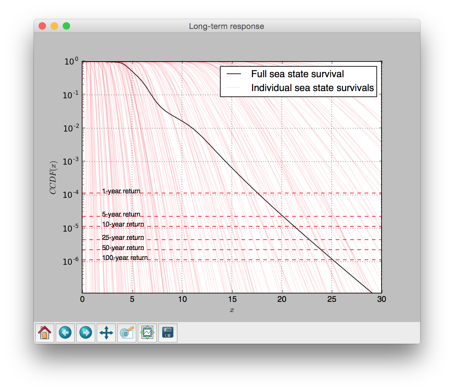
_images/example_longTermFullSeaState.png

Long term complementary cumulative distribution function (CCDF).¶

Fatigue analysis ¶

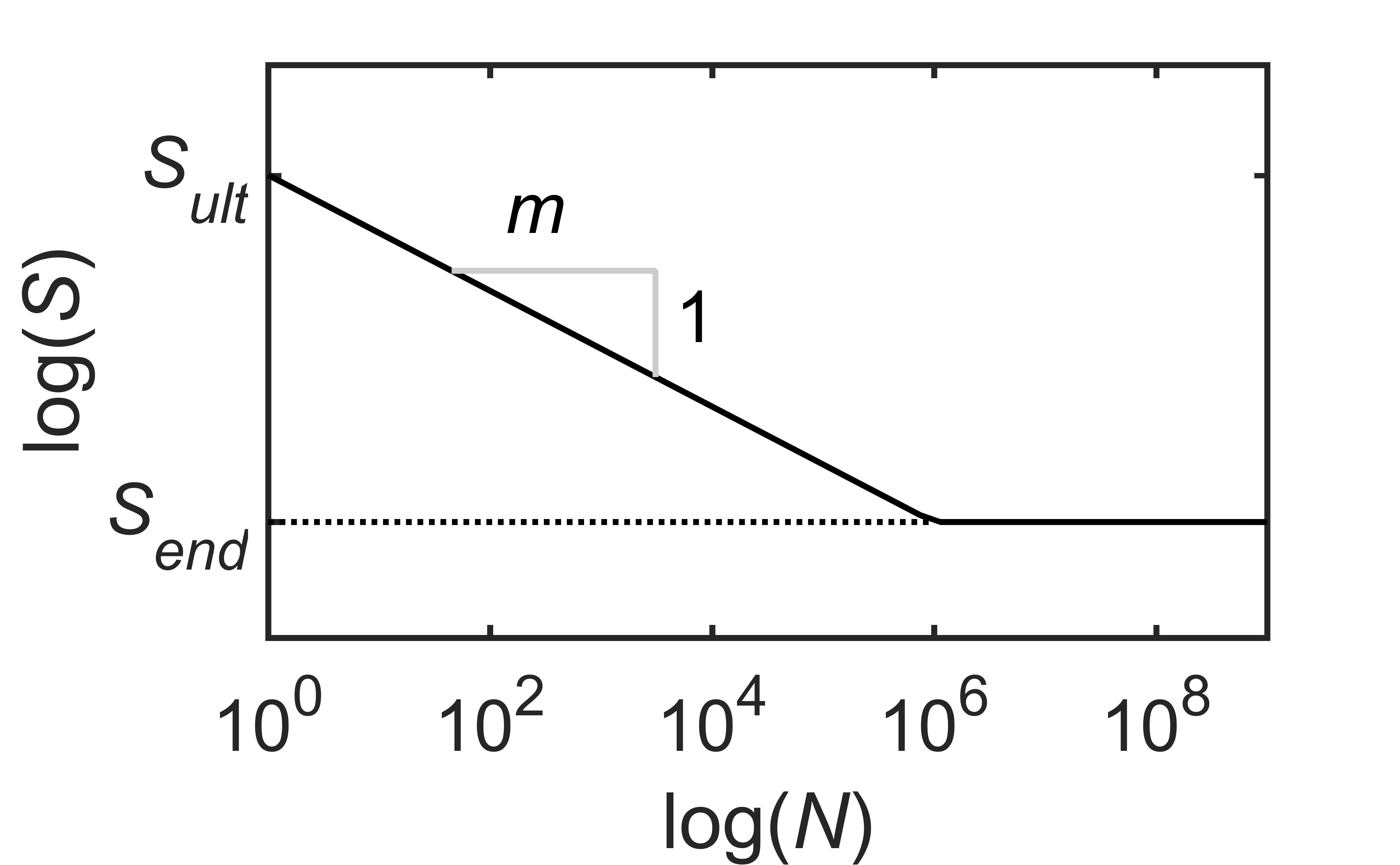
In addition to extreme loads, a WEC must also be able to structurally withstand fatigue loading for its design life. Fatigue loads are time varying loads which cause cumulative damage to structural components and eventually lead to structural failure. Usually, a component’s fatigue strength/life is reported in terms of an $S$-$N$ curve. The $S$-$N$ curve, which is typically obtained empirically, gives the number of load cycles $N$ to failure at constant load amplitude $S$, as illustrated in the following figure. Mathematically, the behavior is described as, $\log (N) = \log (K – m) \log (S)$. Where, $S_{ult}$, is the ultimate strength; $S_{end}$, is the endurance limit, below which, no failure occurs with constant amplitude loading; $m$ is the slope of the $S$-$N$ curve; and, $K$ is an empirical material constant determining the level of the $S$-$N$ curve.

WEC loads, however, are highly variable and by no means of constant amplitude. The most common method used to predict the cumulative damage of variable loading is the Palmgren-Miner rule, as given below. The Palmgren-Miner rule is based on the assumption that the cumulative damage of each load cycle is sequence independent, and thus the total damage equivalent load, $S_{N}$, is obtained with a linear summation of the distributed load ranges. $S_{i}$, the load range for bin $i$, and $n_i$, the number of cycles in load range $i$, are usually obtained via the rain-flow counting method.

\[S_N = \left(\sum{\frac{S^m_i n_i}{N}}\right)^{\frac{1}{m}}\]

The intended used of the fatigue module in the WDRT is as an early design stage WEC fatigue load estimator. The required inputs to the module are:

A force or stress history, which may be obtained either experimentally or via simulation. Pertinent loads may include, power-take-off (PTO) loads, mooring loads, bending moments, etc.

The $S$-$N$ curve slope, $m$, which is likely unknown with any accuracy in the early stages of design, but as an initial estimate, the following ranges may be used: $m \approx 3-4$ for welded steel, $m \approx 6-8$ for cast iron, and $m \approx 9-12$ for composites.

And, $N$, the number of cycles expected in the WEC’s design life, which is up to the user to ascertain given a specified design life and environmental characterization.

This example is shown below and can found in $WDRT_SOURCE/examples/example_fatigue.py.

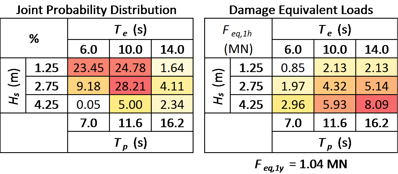
In this example, 1 hour PTO force histories (for the RM3 WEC) have been numerically obtained (using WEC-Sim) for each sea state in the hypothetical joint probability distribution shown below. The average number of cycles expected in 1 hour, $N_{\textrm{1-hr}}$, and 1 year, $N_{\textrm{1-yr}}$, timeframes are estimated from the joint probability distribution. The $S$-$N$ curve slope, $m$, is set to 6. Then, for each sea state, the force histories are read, and using the WDRT fatigue module, 1 hour damage equivalent loads are calculated, as given below. And finally, the annual damage equivalent load is calculated by reapplying the Palmgren-Miner rule and taking advantage of the fact that the rainflow counts were already obtained in the 1 hour damage equivalent load computations, and only need to be adjusted and summed according to the probability of occurrence at each sea state.

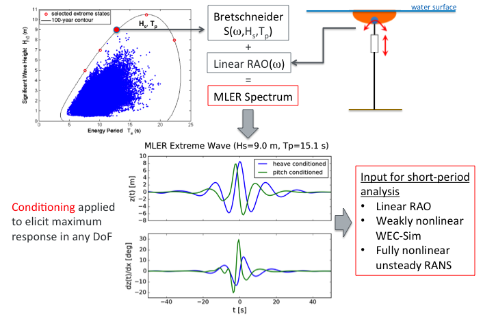
Most-likely extreme response (MLER)¶

The extreme load is often a matter of chance created by the instantaneous position of the device and a series of random waves. The occurrence of an extreme load should be studied as a stochastic event because of the nature of the irregular sea states. The MLER toolbox were developed to generate a focused wave profile that gives the largest response with the consideration of wave statistics based on spectral analysis and the response amplitude operators (RAOs) of the device.

An example can be found in $WDRT_SOURCE/examples/example_MLER_testrun.py.

In this example, the MLER method was applied to model a floating ellipsoid (Quon et al. OMAE 2016). The waves were generated from the extreme wave statistics data and the linear RAOs were obtained from a simple radiation-and-diffraction-method-based numerical model known as the Wave Energy Converter Simulator, or WEC- Sim.

The figure below explains how the MLER waves were generated and used. For this particular example, the target sea state has a significant wave height of 9 m and energy period of 15.1 sec and was represented using Brettschneider spectrum. A specific wave profile is required for different responses of interest (e.g., motion, mooring load, shear stress and bending moment). For example, the MLER wave profile targeting maximum pitch motion is different from the profile for heave, as seen below in the “heave conditioned” and “pitch conditioned” curves. This is expected because the maximum heave and pitch are most likely to occur at different times.