Overview

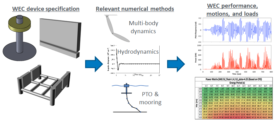
Modeling wave energy converters (WECs) involves the interaction between the incident waves, device motion, power-take-off (PTO mechanism), and mooring. WEC-Sim uses a radiation and diffraction method [B1, B2] to predict power performance and design optimization. The radiation and diffraction method generally obtains the hydrodynamic forces from a frequency-domain boundary element method (BEM) solver using linear coefficients to solve the system dynamics in the time domain.

Coordinate System

The WEC-Sim Coordinate System figure illustrates a 3-D floating point absorber subject to incoming waves in water. The figure also defines the coordinates and the 6 degree of freedom (DOF) in WEC-Sim. The WEC-Sim coordinate system assumes that the positive X-axis defines a wave angle heading of zero (e.g., a wave propagating with along a zero-degree direction is moving in the +X direction). The positive Z-axis is in the vertical upwards direction, and the positive Y-axis direction is defined by the right-hand rule. In the vectors and matrices used in the code, Surge (x), Sway (y), and Heave (z) correspond to the first, second and third position respectively. Roll (Rx), Pitch (Ry), and Yaw (Rz) correspond to the fourth, fifth, and sixth position respectively.

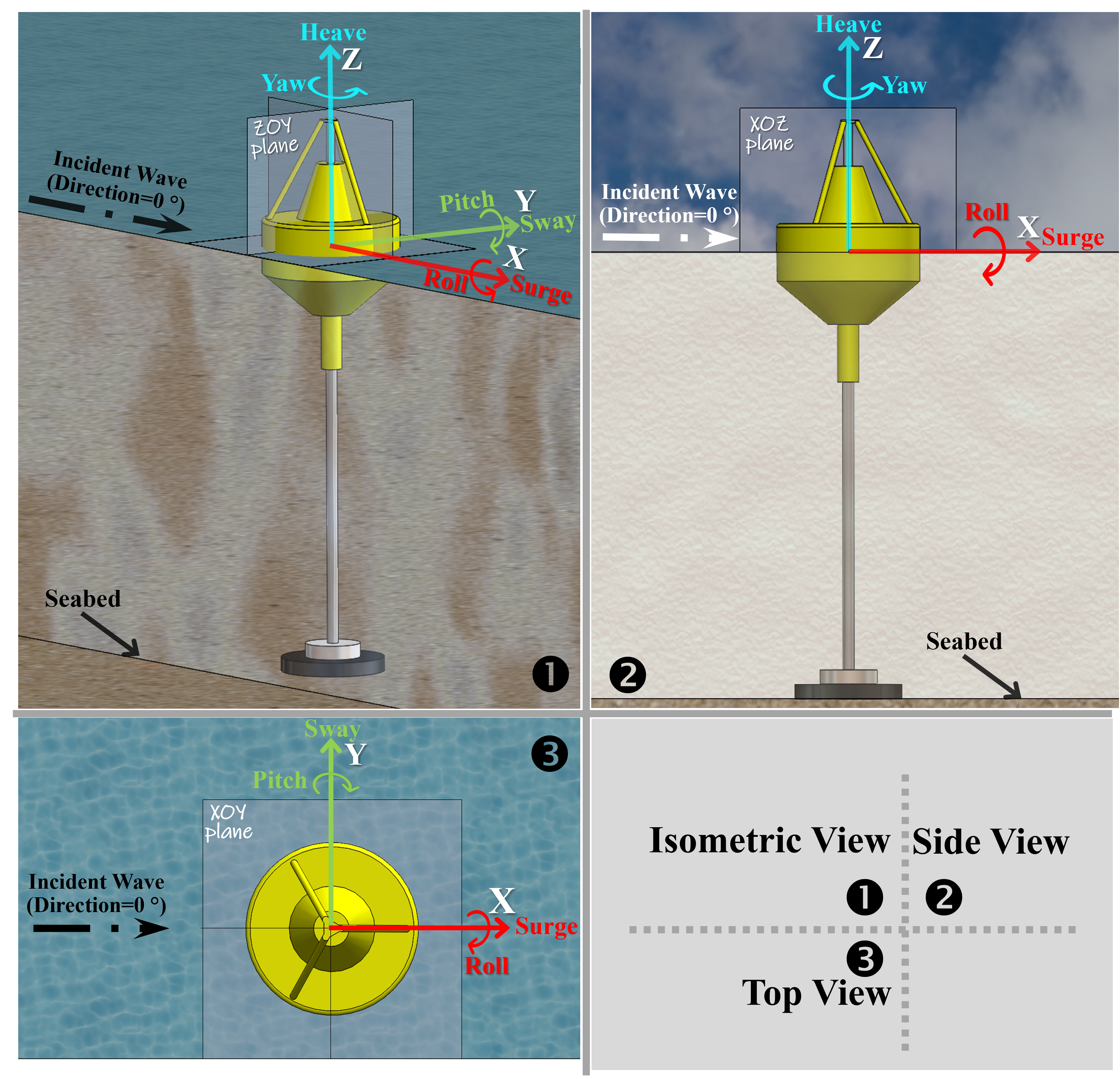
WEC-Sim Coordinate System

Units

All units within WEC-Sim are in the MKS (meters-kilograms-seconds system) and angular measurements are specified in radians (except for wave directionality which is defined in degrees).

Boundary Element Method (BEM)

In WEC-Sim, wave forcing components are modeled using linear coefficients obtained from a frequency-domain potential flow Boundary Element Method (BEM) solver (e.g., WAMIT [B3], Aqwa [B4], NEMOH [B5], and Capytaine [B6, B7]). The BEM solutions are obtained by solving the Laplace equation for the velocity potential, which assumes the flow is inviscid, incompressible, and irrotational. More details on the theory for the frequency-domain BEM can be found in [B3].

WEC-Sim imports nondimensionalized hydrodynamic coefficients from an *.h5 data structure generated by BEMIO for the BEM solvers: WAMIT, Aqwa, NEMOH or Capytaine. Alternatively, the *.h5 data structure can be manually defined by the user. The WEC-Sim code scales the hydrodynamic coefficients according to the equations below, where \(\rho\) is the water density, \(\omega\) is the wave frequency in rad/s, and \(g\) is gravity:

\begin{gather*} |\overline{F_{exc}(\omega)}| = \frac{|F_{exc}(\omega)|}{\rho g} \\ \overline{A(\omega)} = \frac{A(\omega)}{\rho} \\ \overline{B(\omega)} = \frac{B(\omega)}{\rho \omega} \\ \overline{K_{hs}} = \frac{K_{hs}}{\rho g} \end{gather*}

where \(F_{exc}\) is the wave-excitation force and torque vector, \(A\) is the radiation added mass coefficient, \(B\) is the radiation wave damping coefficient, and \(K_{hs}\) is the linear hydrostatic restoring coefficient.

Time-Domain Formulation

A common approach to determining the hydrodynamic forces is to use linear wave theory which assumes the waves are the sum of incident, radiated, and diffracted wave components. The dynamic response of the system is calculated by solving WEC system equations of motion [B2, B8]. The equation of motion for a floating body about its center of gravity can be given as:

\[m\ddot{X}=F_{exc}(t)+F_{md}(t)+F_{rad}(t)+F_{pto}(t)+F_{v}(t)+F_{me}(t)+F_{B}(t)+F_{m}(t)\]

where \(\ddot{X}\) is the (translational and rotational) acceleration vector of the device, \(m\) is the mass matrix, \(F_{exc}(t)\) is the wave excitation force and torque (6-element) vector, \(F_{md}(t)\) is the mean drift force and torque vector, \(F_{rad}(t)\) is the force and torque vector resulting from wave radiation, \(F_{pto}(t)\) is the PTO force and torque vector, \(F_{v}(t)\) is the damping force and torque vector, \(F_{me}(t)\) is the Morison Element force and torque vector, \(F_{B}(t)\) is the net buoyancy restoring force and torque vector, and \(F_{m}(t)\) is the force and torque vector resulting from the mooring connection.

\(F_{exc}(t)\) , \(F_{rad}(t)\) , and \(F_{B}(t)\) are calculated using hydrodynamic coefficients provided by the frequency-domain BEM solver. The radiation term includes an added-mass term, matrix \(A(\omega)\), and wave damping term, matrix \(B(\omega)\), associated with the acceleration and velocity of the floating body, respectively, and given as functions of radian frequency (\(\omega\)) by the BEM solver. The wave excitation term \(F_{exc}(\omega)\) includes a Froude-Krylov force component generated by the undisturbed incident waves and a diffraction component that results from the presence of the floating body. The buoyancy term \(F_{B}(t)\) depends on the hydrostatic stiffness \(K_{hs}\) coefficient, displacement of the body, and its mass.

Numerical Methods

WEC-Sim can be used for regular and irregular wave simulations, but note that \(F_{rad}(t)\) is calculated differently for sinusoidal steady-state response scenarios and random sea simulations. The sinusoidal steady-state response is often used for simple WEC designs with regular incoming waves. However, for random sea simulations or any simulations where fluid memory effects of the system are essential, the convolution integral method is recommended to represent the fluid memory retardation force on the floating body. To speed computation of the convolution integral, the state space representation method can be specified to approximate this calculation as a system of linear ordinary differential equations.

Ramp Function

A ramp function (\(R_{f}\)), necessary to avoid strong transient flows at the earlier time steps of the simulation, is used to calculate the wave excitation force. The ramp function is given by

\[\begin{split}R_{f}(t)=\begin{cases} \frac{1}{2}(1+\cos(\pi+\frac{\pi t}{t_{r}})) & \frac{t}{t_{r}}<1\\ 1 & \frac{t}{t_{r}}\geq1 \end{cases}\end{split}\]

where \(t\) is the simulation time and \(t_{r}\) is the ramp time.

Sinusoidal Steady-State Response

This approach assumes that the system response is in sinusoidal steady-state form; therefore, it is only valid for regular wave simulations. The radiation term can be calculated using the added mass and the wave radiation damping term for a given wave frequency, which is obtained from

\[F_{rad}(t)=-A(\omega)\ddot{X}-B(\omega)\dot{X}\]

where \(\dot{X}\) is the velocity vector of the floating body, \(A(\omega)\) is the added mass matrix, and \(B(\omega)\) is the radiation damping matrix.

The free surface profile is based on linear wave theory for a given wave height, wave frequency, and water depth. The regular wave excitation force is obtained from

\[F_{exc}(t)=\Re\left[ R_{f}(t)\frac{H}{2}F_{exc}(\omega, \theta)e^{i\omega t} \right]\]

where \(\Re\) denotes the real part of the formula, \(R_{f}\) is the ramp function, \(H\) is the wave height, \(F_{exc}\) is the frequency dependent complex wave-excitation amplitude vector, and \(\theta\) is the wave direction.

The mean drift force has two contributions:

• 2nd-order hydrodynamic pressure due to the first-order wave

• Interaction between the first-order motion and the first-order wave

Currently, WEC-Sim only reads mean drift coefficients representing the first contribution. The mean drift force can optionally be included if these coefficients are defined in the BEM data. The mean drift force is obtained from:

\[F_{md}(t)=\left(\frac{H}{2}\right)^2F_{md}(\omega,\theta)\]

The mean drift force is combined with the excitation force in the response class output.

Note

Currently, WEC-Sim only supports mean drift coefficients from WAMIT.

Convolution Integral Formulation

In the case of an irregular wave spectrum, the fluid memory has an important impact on the WEC dynamics. This fluid memory effect is captured by the convolution integral formulation based upon the Cummins equation [B9] is used. The radiation term can be calculated by

\[F_{rad}(t)=-A_{\infty}\ddot{X}-\intop_{0}^{t}K_{r}(t-\tau)\dot{X}(\tau)d\tau\]

where \(A_{\infty}\) is the added mass matrix at infinite frequency and \(K_{r}\) is the radiation impulse response function. This representation also assumes that there is no motion for \(t<0\). The radiation impulse response function is defined as

\[K_{r}(t) = \frac{2}{\pi} \intop_{0}^{\infty} B(\omega) cos(\omega t) d\omega\]

For regular waves, the equation described in the last subsection is used to calculate the wave excitation vector. For irregular waves, the free surface elevation is constructed from a linear superposition of a number of regular wave components. Each regular wave component is extracted from a wave spectrum, \(S(\omega)\), describing the wave energy distribution over a range of wave frequencies, generally characterized by a significant wave height and peak wave period. The irregular excitation force can be calculated as the real part of an integral term across all wave frequencies as follows

\[F_{exc}(t)=\Re\left[ R_{f}(t) \sum_{j=1}^{N} F_{exc}(\omega_{j}, \theta) e^{i(\omega_{j}t+\phi_{j})} \sqrt{2S(\omega_{j})d\omega_{j}} \right]\]

where \(\phi\) is the randomized phase angle and \(N\) is the number of frequency bands selected to discretize the wave spectrum. For repeatable simulation of an irregular wave field \(S(\omega)\), WEC-Sim allows specification of \(\phi\), refer to the Multiple Wave-Spectra section.

Additionally, an excitation force impulse response function is defined as

\[K_{e}(t) = \frac{1}{2\pi} \intop_{-\infty}^{\infty} F_{exc}(\omega,\theta)e^{i\omega t} d\omega\]

The excitation impulse response function is only used for the userDefinedElevation wave case.

State Space

It is highly desirable to represent the radiation convolution integral described in the last subsection in state space (SS) form [B10]. This has been shown to dramatically increase computational speeds [B11] and allow utilization of conventional control methods that rely on linear state space models. An approximation will need to be made as \(K_{r}\) is solved from a set of partial differential equations where as a linear state space is constructed from a set of ordinary differential equations. In general, a linear system is desired such that:

\[\begin{split}\dot{X}_{r} \left( t \right) = \mathbf{A_{r}} X_{r} \left( t \right) + \mathbf{B_{r}} \mathbf{u} (t);~~X_{r}\left( 0 \right) = 0~~ \nonumber \\ \int_{0}^{t} \mathbf{K_{r}} \left( t- \tau \right) d\tau \approx \mathbf{C_{r}} X_{r} \left( t \right) + \mathbf{D_{r}} \mathbf{u} \left( t \right)~~\end{split}\]

with \(\mathbf{A_{r}},~\mathbf{B_{r}},~\mathbf{C_{r}},~\mathbf{D_{r}}\) being the time-invariant state, input, output, and feed through matrices, while \(u\) is the input to the system and \(X_{r}\) is the state vector describing the convolution kernel as time progresses.

Calculation of \(K_{r}\) from State Space Matrices

The impulse response of a single-input zero-state state-space model is represented by

\[\begin{split}\dot{x} &= \mathbf{A_{r}} x + \mathbf{B_{r}} u \\ y &= \mathbf{C_{r}} x\end{split}\]

where \(u\) is an impulse. If the initial state is set to \(x(0)= \mathbf{B_{r}} u\) the response of the unforced (\(u=0\)) system

\[\begin{split}\dot{x} &= \mathbf{A_{r}} x \\ y &= \mathbf{C_{r}} x\end{split}\]

is clearly equivalent to the zero-state impulse response. The impulse response of a continuous system with a nonzero \(\mathbf{D_r}\) matrix is infinite at \(t=0\); therefore, the lower continuity value \(\mathbf{C_{r}}\mathbf{B_{r}}\) is reported at \(t=0\). The general solution to a linear time invariant (LTI) system is given by:

\[x(t) = e^{\mathbf{A_{r}}t} x(0) + \int_{0}^{t} e^{\mathbf{A_{r}}(t-\tau)} \mathbf{B_{r}} u (\tau) d\tau~~\]

where \(e^{\mathbf{A_{r}}}\) is the matrix exponential and the calculation of \(K_{r}\) follows:

\[K_{r}(t) = \mathbf{C_{r}}e^{\mathbf{A_{r}}t}\mathbf{B_{r}}~~\]

Realization Theory

The state space realization of the hydrodynamic radiation coefficients can be pursued in the time domain (TD). This consists of finding the minimal order of the system and the discrete time state matrices (\(\mathbf{A_{d}},~\mathbf{B_{d}},~\mathbf{C_{d}},~\mathbf{D_{d}}\)) from samples of the impulse response function. This problem is easier to handle for a discrete-time system than for continuous-time. The reason being is that the impulse response function of a discrete-time system is given by the Markov parameters of the system:

\[\mathbf{\tilde{K}_{r}} \left( t_{k} \right) = \mathbf{C_{d}}\mathbf{A_{d}}^{k}\mathbf{B_{d}}~~\]

where \(t_{k}=k\Delta t\) for \(k=0,~1,~2,~\ldots\) with \(\Delta t\) being the sampling period. The feedthrough matrix \(\mathbf{D_d}\) is assumed to be zero in order to maintain causality of the system, as a non-zero \(\mathbf{D_d}\) results in an infinite value at \(t=0\).

The most common algorithm to obtain the realization is to perform a Singular Value Decomposition (SVD) on the Hankel matrix of the impulse response function, as proposed by Kung [B12]. The order of the system and state-space parameters are determined from the number of significant singular values and the factors of the SVD. The Hankel matrix (\(H\)) of the impulse response function

\[\begin{split}H = \begin{bmatrix} \mathbf{K_{r}}(2) & \mathbf{K_{r}}(3) & \ldots & \mathbf{K_{r}}(n) \\ \mathbf{K_{r}}(3) & \mathbf{K_{r}}(4) & \ldots & 0 \\ \vdots & \vdots & \ddots & \vdots \\ \mathbf{K_{r}}(n) & 0 & \cdots & 0 \end{bmatrix} &\\\end{split}\]

can be reproduced exactly by the SVD as

\[H = \mathbf{U} \Sigma \mathbf{V^{*}}\]

where \(\Sigma\) is a diagonal matrix containing the Hankel singular values in descending order. Examination of the Hankel singular values reveals there are only a small number of significant states and that the rank of \(H\) can be greatly reduced without a significant loss in accuracy [B11, B13]. Further detail into the SVD method and calculation of the state space parameters will not be discussed here and the reader is referred to [B11, B13].

Regular Waves

Regular waves are defined as planar sinusoidal waves, where the incident wave is defined as \(\eta(x,y,t)\) :

\[\eta(x,y,t)= \frac{H}{2} \cos( \omega t - k (x\cos \theta + y\sin \theta) + \phi)\]

where \(H\) is the wave height, \(\omega\) is the wave frequency (\(\omega = \frac{2\pi}{T}\)), \(k\) is the wave number (\(k = \frac{2\pi}{\lambda}\)), \(\theta\) is the wave direction, and \(\phi\) is the wave phase.

Dispersion Relation

For ocean waves, the dispersion relation is a relation between the wave angular frequency and the wave number (i.e. wavelength). The dispersion relation is derived using separation of variables to satisfy the free surface kinematic and dynamic boundary conditions. For a more detailed derivation please the reader is referred here The dispersion relation that WEC-sim uses is defined as:

\[\begin{split}\omega^{2} = gk\tanh\left(kh\right) \approx \begin{cases} gk & \text{as } kh \rightarrow \infty \\ gk^{2}h & \text{as } kh \rightarrow 0 \end{cases}\end{split}\]

where \(\omega\) is the wave angular frequency (\(\omega = \frac{2\pi}{T}\)), \(g\) is gravitational acceleration, \(k\) is the wave number (\(k=\frac{2\pi}{\lambda}\)), and \(h\) is the water depth. The dispersion relation can be simplified if the floating body is located in deep water, \(h \rightarrow \infty\) . The simplification comes from the hyperbolic tangent function having an asympote of 1 as its argument tends to infinity (\(\tanh \left( \infty \right) \rightarrow 1\)). The deep water condition can still be met if the water depth is not infinite while the following expression holds \(kh \geq \pi\) . The dispersion relation can then be used to derive the phase velocity which refers to the speed that an observer would need to travel for the wave to appear stationary (unchanging). The phase velocity of a two-dimensional progressive wave is given by the following expression:

\[\begin{split}c_{p} = \frac{\omega}{k} = \sqrt{\frac{g}{k}\tanh\left(kh\right)} \approx \begin{cases} \sqrt{\frac{g}{k}}=\frac{g}{\omega} & \text{as } kh \rightarrow \infty \\ \sqrt{gh} & \text{as } kh \rightarrow 0 \end{cases}\end{split}\]

Regular Wave Power

The time-averaged power, per unit wave crest with, for a propagating water wave

\[P_{w} = \frac{1}{2}\rho g A^{2} c_{g}\]

where \(\rho\) is the fluid density, \(g\) is gravitational acceleration, \(A\) is the wave amplitude, and \(c_{g}\) is wave group velocity. The group velocity is the speed of propagation of a packet of waves which is always slower than the wave phase velocity. For a more detailed derivation on the group velocity the reader is referred here. The group velocity of a two-dimensional progressive wave is given by the following expression:

\[c_{g} = \frac{\delta \omega}{\delta k} = \frac{1}{2} \sqrt{\frac{g}{k}\tanh\left(kh\right)} \left( 1 + \frac{2kh}{\sinh \left( 2kh \right)} \right)\]

where \(\sinh\) is the hyperbolic sine function. The square root term is the phase velocity which can be used to simplify the group velocity expression as follows:

\[\begin{split}c_{g} = \frac{1}{2} c_{p} \left( 1 + \frac{2kh}{\sinh \left( 2kh \right)} \right) \approx \begin{cases} \frac{1}{2} c_{p} & \text{as } kh \rightarrow \infty \\ 1 & \text{as } kh \rightarrow 0 \end{cases}\end{split}\]

Inserting the full expression for the group velocity into the wave power equation provides the following:

\[P_{w} = \frac{1}{4}\rho g A^{2} \sqrt{\frac{g}{k}\tanh\left(kh\right)} \left[ 1 + \frac{2kh}{\sinh \left( 2kh \right)} \right]\]

Similar to the other wave property expressions, the wave power expression can be simplified for both deep and shallow water conditions as follows:

\[\begin{split}P_{w} \approx \begin{cases} \frac{1}{4}\rho g A^{2} \sqrt{\frac{g}{k}} = \frac{1}{8\pi}\rho g^{2} A^{2} T & \text{as } kh \rightarrow \infty \\ \frac{1}{4}\rho g A^{2} \sqrt{gh} & \text{as } kh \rightarrow 0 \end{cases}\end{split}\]

Note

The deep water condition is often used without proper validation of the wave environment which can have a significant effect on wave power. WEC-Sim by default will calculate the wave power using the full expression, no simplification, unless the hydrodynamic data is imported with the assumption of infinite water depth.

Irregular Waves

Irregular waves are modeled as the linear superposition of a large number of harmonic waves at different frequencies and angles of incidence, where the incident wave is defined as \(\eta(x,y,t)\) :

\[\eta(x,y,t) = \sum_{i} \frac{H_{i}}{2} \cos( \omega_{i} t - k_{i} (x\cos \theta_{i} + y \sin \theta_{i}) + \phi_{i})\]

where \(H\) is the wave height, \(\omega\) is the wave frequency (\(\omega = \frac{2\pi}{T}\)), \(k\) is the wave number (\(k = \frac{2\pi}{\lambda}\)), \(\theta\) is the wave direction, and \(\phi\) is the wave phase (randomized for irregular waves).

Wave Spectra

The linear superposition of regular waves of distinct amplitudes and periods is characterized in the frequency domain by a wave spectrum. Through statistical analysis, spectra are characterized by specific parameters such as significant wave height, peak period, wind speed, fetch length, and others. Common types of wave spectra that are used by the offshore industry are discussed in the following sections. The general form of the wave spectra available in WEC-Sim is given by:

\[S\left( f , \theta \right)= S\left( f \right)D\left( \theta \right)~~\]

where \(S\left( f\right)\) is the wave power spectrum, \(f\) is the wave frequency (in Hertz), \(D\left( \theta \right)\) is the directional distribution, and \(\theta\) is the wave direction (in Degrees). The formulation of \(D\left( \theta \right)\) requires that

\[\int_{0}^{\infty} \int_{-\pi}^{\pi} S \left( f \right) D \left( \theta \right) d\theta df = \int_{0}^{\infty} S\left( f \right) df\]

so that the total energy in the directional spectrum must be the same as the total energy in the one-dimensional spectrum.

\[S\left( f \right) = A_{ws} f^{-5}\exp\left[-B_{ws} f^{-4} \right]~~\]

where \(A_{ws}\) and \(B_{ws}\) are coefficients that vary depending on the wave spectrum and \(\exp\) stands for the exponential function. Spectral moments of the wave spectrum, denoted \(m_{k}~,~k=0, 1, 2,...\), are defined as

\[m_{k} = \int_{0}^{\infty} f^{k} S \left( f \right) df ~~\]

The spectral moment, \(m_{0}\) is the variance of the free surface which allows one to define the mean wave height of the tallest third of waves, significant wave height \(H_{m0}\) (in m), as:

\[H_{m0} = 4 \sqrt{m_{0}}~~\]

Irregular Wave Power

The time-averaged wave power available for a given irregular sea state can be calcuated from:

\[P_{w} = \rho g \int_{0}^{\infty} S \left( f \right) c_{g} \left( f \right) df\]

where the expression for group velocity for regular waves can be inserted for each frequency used to describe the sea spectrum.

Pierson–Moskowitz (PM) Spectrum

The PM spectrum is applicable to a fully developed sea, when the growth of the waves is not limited by the fetch [B14]. The two-parameter PM spectrum is based on a significant wave height and peak wave frequency. For a given significant wave height, the peak frequency can be varied to cover a range of conditions including developing and decaying seas. In general, the parameters depend strongly on wind speed, and also wind direction, fetch, and locations of storm fronts. The spectral density of the surface elevation defined by the PM spectrum [B15] is defined by:

\[S_{PM}\left( f \right) = \frac{{H_{m0}}^2}{4} \left( 1.057f_{p} \right)^{4} f^{-5} \exp \left[-\frac{5}{4} \left( \frac{f_{p}}{f}\right)^{4} \right]\]

This implies coefficients of the general form:

\[\begin{split}A_{ws} &= \frac{{H_{m0}}^2}{4}\left(1.057f_{p}\right)^{4} \approx \frac{5}{16} {H_{m0}}^2 {f_{p}}^{4} \approx \frac{B_{ws}}{4}{H_{m0}}^2 \\ B_{ws} &= \left(1.057f_{p}\right)^{4} \approx \frac{5}{4}{f_{p}}^{4}\end{split}\]

where \(H_{m0}\) is the significant wave height, \(f_{p}\) is the peak wave frequency \(\left(=1/T_{p}\right)\), and \(f\) is the wave frequency.

JONSWAP (JS) Spectrum

The JONSWAP (Joint North Sea Wave Project) spectrum is formulated as a modification of the PM spectrum for developing sea sate in a fetch-limited situation [B16]. The spectrum accounts for a higher peak and a narrower spectrum in a storm situation for the same total energy as compared to the PM spectrum. The spectral density of the surface elevation defined by the JS spectrum [B15] is defined by:

\[S_{JS}\left( f \right) = C_{ws} \left(\gamma\right) S_{PM} \gamma^{\alpha}\]

where \(\gamma\) is the nondimensional peak-shape parameter.

The normalizing factor, \(C_{ws}\left(\gamma\right)\), is defined as:

\[C_{ws}\left(\gamma\right) = \frac{\int_{0}^{\infty} S_{PM}\left( f \right)df} {\int_{0}^{\infty}S_{PM}\left(f\right)\gamma^{\alpha}df} = 1 -0.287\ln\left(\gamma\right)\]

The peak-shape parameter exponent \(\alpha\) is defined as:

\[\begin{split}\alpha = \exp \left[ -\left( \frac{\frac{f}{f_{p}}-1}{\sqrt{2} \sigma}\right)^{2} \right],~~ \sigma = \begin{cases} 0.07 & f \leq f_{p} \\0.09 & f > f_{p} \end{cases} ~~\end{split}\]

The peak-shape parameter is defined based on the following relationship between the significant wave height, \(H_{m0}\), and peak period, \(T_{p}\):

\[\begin{split}\gamma = \begin{cases} 5 & \text{for } \frac{T_{p}}{\sqrt{H_{m0}}} \leq 3.6 \\ \exp\left(5.75 - 1.15\frac{T_{p}}{\sqrt{H_{m0}}} \right) & \text{for } 3.6 \leq \frac{T_{p}}{\sqrt{H_{m0}}} \leq 5 \\ 1 & \text{for } \frac{T_{p}}{\sqrt{H_{m0}}} > 5 \end{cases}\end{split}\]

with general form coefficients thus defined:

\[\begin{split}A_{ws} &= \frac{B_{ws}}{4}{H_{m0}}^2 C_{ws}\left(\gamma \right) \gamma^{\alpha} \\ B_{ws} &= \frac{5}{4}{f_{p}}^{4}\end{split}\]

Ocean Current

An ocean current is a continuous, directed movement of sea water generated by a number of forces acting upon the water, including wind, the Coriolis effect, breaking waves, cabbeling, temperature and salinity differences, and other ocean phenomena. Depth contours, shoreline configurations, and interactions with other currents influence a current’s direction and strength. Ocean current can vary in space and time, but are generally modeled assuming a horizontally uniform flow field of constant velocity and direction, varying only as a function of depth.

Ocean Current Profiles Within WEC-Sim

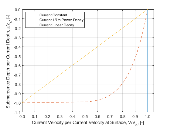
Within WEC-Sim there are three options to model ocean currents:

Option 1

In Option 1, the sub-surface current is depth independent and is equal to the current at the water surface:

\[\vec{U}_{ss,current}(z) = U_{ss,current}(0)\left[ \cos \left(\theta_{c} \right) \hat{i} + \sin \left(\theta_{c} \right) \hat{j} \right]\]

where \(\theta_{c}\) is the current direction.

Option 2

In Option 2, the sub-surface current profile varies with depth following a 1/7th power law:

\[\vec{U}_{ss,current}(z) = U_{ss,current}(0)\left[ 1 + \frac{z}{d_{current}} \right]^{1/7} \left[ \cos \left(\theta_{c}\right) \hat{i} + \sin \left(\theta_{c} \right) \hat{j} \right]\]

where \(d_{current}\) is the water depth where the sub-surface current is 0.

Option 3

In Option 3, the sub-surface current profile varies linearly with depth:

\[\vec{U}_{ss,current}(z) = U_{ss,current}(0)\left[ 1 + \frac{z}{d_{current}} \right] \left[ \cos \left(\theta_{c} \right) \hat{i} + \sin \left(\theta_{c} \right) \hat{j} \right]\]

Note

WEC-Sim does not adjust the linear wave hydrodynamics based on the presence of ocean currents and assumes a linear superposition between current and wave forces. The ocean current option is used only in the Morison Element force calculation.

Power Take-Off (PTO)

Throughout the following sections, unless specification is made between linear and rotary PTOs, units are not explicitly stated.

Linear PTO

The PTO mechanism is represented as a linear spring-damper system where the reaction force is given by:

\[F_{pto}=-K{}_{pto}X_{rel}-C_{pto}\dot{X}_{rel}\]

where \(K_{pto}\) is the stiffness of the PTO, \(C_{pto}\) is the damping of the PTO, and \(X_{rel}\) and \(\dot{X}_{rel}\) are the relative motion and velocity between two bodies. The instantaneous power absorbed by the PTO is given by:

\[P_{pto} = -F_{pto}\dot{X}_{rel} = \left(K_{pto}X_{rel} \dot{X}_{rel} + C_{pto} \dot{X}^{2}_{rel} \right)\]

Hydraulic PTO

The PTO mechanism is modeled as a hydraulic system [B17], where the reaction force is given by:

\[F_{pto}=\Delta{} p_{piston}A_{piston}\]

where \(\Delta{} p_{piston}\) is the differential pressure of the hydraulic piston and \(A_{piston}\) is the piston area. The instantaneous hydraulic power absorbed by the PTO is given by:

\[P_{pto}=-F_{pto}\dot{X}_{rel}\]

Mechanical PTO

The PTO mechanism is modeled as a direct-drive linear generator system [B17], where the reaction force is given by:

\[F_{pto}=(\frac{\pi}{\tau_{pm}})\lambda_{fd}i_{sq}\]

where \(\tau_{pm}\) is the magnet pole pitch (the center-to-center distance of adjacent magnetic poles), \(\lambda_{fd}\) is the flux linkage of the stator \(d\)-axis winding due to flux produced by the rotor magnets, and \(i_{sq}\) is the stator \(q\)-axis current. The instantaneous mechanical power absorbed by the PTO is given by:

\[P_{pto}=-F_{pto}\dot{X}_{rel}\]

For more information about application of pto systems in WEC-Sim, refer to Constraint and PTO Features section.

Mooring

The mooring load is represented using a linear quasi-static mooring stiffness or by using the mooring forces calculated from MoorDyn [B18], which is an open-source lumped-mass mooring dynamics model.

Mooring Matrix

When linear quasi-static mooring stiffness is used, the mooring load can be calculated by

\[F_{m}=-K_{m}X-C_{m}\dot{X}\]

where \(K_{m}\) and \(C_{m}\) are the stiffness and damping matrices for the mooring system, and \(X\) and \(\dot{X}\) are the displacement and velocity of the body, respectively.

Mooring Lookup Table

The Mooring Lookup Table searches a user-supplied 6DOF force lookup table. The lookup table must contain six parameters: the resultant mooring force in each degree of freedom. Each force must be indexed by position in all six degrees of freedom, as shown below. The mooringClass does not assume a value for empty indices or forces. All degrees of freemdom must be initialized and supplied by the user. The mooring force is linearly interpolated between indexed positions based on the instantaneous position of the mooring system using a Simulink N-D Lookup Table for each force component. The fidelity of the mooring lookup table is entirely dependent on the user-defined input.

MoorDyn

MoorDyn discretizes each mooring line in a mooring system into evenly-sized line segments connected by node points (see MoorDyn figure). The line mass is lumped at these node points along with gravitational and buoyancy forces, hydrodynamic loads, and reactions from contact with the seabed. Hydrodynamic drag and added mass are calculated based on Morison’s equation. A mooring line’s axial stiffness is modeled by applying a linear stiffness to each line segment in tension only. A damping term is also applied in each segment to dampen non-physical resonance caused by the lumped-mass discretization. Bending and torsional stiffnesses are neglected. Bottom contact is represented by vertical stiffness and damping forces applied at the nodes when a node is located below the seabed. [B19].

MoorDyn mooring model elements

For more information about application of mooring systems in WEC-Sim, refer to Mooring Features section.

Nonlinear Buoyancy and Froude-Krylov Wave Excitation

The linear model assumes that the body motion and the waves consist of small amplitudes in comparison to the wavelengths. A weakly nonlinear approach is applied to account for the nonlinear hydrodynamic forces induced by the instantaneous water surface elevation and body position. Rather than using the BEM calculated linear wave-excitation and hydrostatic coefficients, the nonlinear buoyancy and the Froude-Krylov force components can be obtained by integrating the static and dynamic pressures over each panel along the wetted body surface at each time step. Linear wave theory is used to determine the flow velocity and pressure field, so the values become unrealistically large for wetted panels that are above the mean water level. To correct this, the Wheeler stretching method is applied [B20], which applies a correction to the instantaneous wave elevation that forces its height to be equal to the water depth when calculating the flow velocity and pressure,

\[z^* = \frac{D(D+z)}{(D+\eta)} - D\]

where \(D\) is the mean water depth, and \(\eta\) is the z-value on the instantaneous water surface.

Note

The nonlinear WEC-Sim method is not intended to model highly nonlinear hydrodynamic events, such as wave slamming and wave breaking.

For more information about application of nonlinear hydrodynamics in WEC-Sim, refer to Nonlinear Buoyancy and Froude-Krylov Excitation section.

Viscous Damping and Morison Elements

Additional damping and added-mass can be added to the WEC system. This facilitates experimental validation of the WEC-Sim code, particularly in the event that the BEM hydrodynamic outputs are not sufficiently representative of the physical system.

Viscous Damping

Linear damping and quadratic drag forces add flexibility to the definition of viscous forcing

\[\begin{split}F_{v} &= -C_{v}\dot{X}-\frac{C_{d} \rho A_{d}}{2}\dot{X}|\dot{X}| \\ &= -C_{v}\dot{X}-C_{D}\dot{X}|\dot{X}|\end{split}\]

where \(C_{v}\) is the linear (viscous) damping coefficient, \(C_{d}\) is the quadratic drag coefficient, \(\rho\) is the fluid density, and \(A_{d}\) is the characteristic area for drag calculation. Alternatively, one can define \(C_{D}\) directly.

Because BEM codes are potential flow solvers and neglect the effects of viscosity, \(F_{v}\) generally must be included to accurately model device performance. However, it can be difficult to select representative drag coefficients, as they depend on device geometry, scale, and relative velocity between the body and the flow around it. Empirical data on the drag coefficient can be found in various literature and standards, but is generally limited to simple geometries evaluated at a limited number of scales and flow conditions. For realistic device geometries, the use of computational fluid dynamic simulations or experimental data is encouraged.

Morison Elements

The Morison Equation assumes that the fluid forces in an oscillating flow on a structure of slender cylinders or other similar geometries arise partly from pressure effects from potential flow and partly from viscous effects. A slender cylinder implies that the diameter, D, is small relative to the wave length, \(\lambda\), which is generally met when \(D/\lambda < 0.1 - 0.2\). If this condition is not met, wave diffraction effects must be taken into account. Assuming that the geometries are slender, the resulting force can be approximated by a modified Morison formulation [B21]. The formulation for each element on the body can be given as

\[F_{me}=\rho\forall\dot{v} + \rho\forall C_{a}(\dot{v}-\ddot{X}) + \frac{C_{d}\rho A_{d}}{2}(v-\dot{X})|v-\dot{X}|\]

where \(v\) is the fluid particle velocity due to the wave and current speed, \(C_{a}\) is the coefficient of added mass, and \(\forall\) is the displaced volume.

Note

WEC-Sim does not consider buoyancy effects when calculating the forces from Morison elements.

For more information about application of Morison Elements in WEC-Sim, refer to Morison Elements section.

Generalized Body Modes

Additional generalized body modes (GBM) are included to account for solving a multibody system with relative body motions, dynamics, or structural deformation. This implementation assumes the modal properties are given, obtainable in closed-form expressions or with finite element analysis. Once the hydrodynamic coefficients that include these additional flexible DOF are obtained from the BEM solver, the 6DOF rigid body motion for each body and the additional GBM DOFs are solved together in one system of equations. See this example and Advanced Features for more details on implementing GBM.

Terminology

Term or Variable	Definition
\(A(\omega)\)	Frequency dependent radiation added mass and inertia (kg and kg-m^2)
\(\overline{A(\omega)}\)	Normalized frequency dependent radiation added mass
\(A_{\infty}\)	Added mass and inertia at infinite frequency (kg and kg-m^2)
\(A_{d}\)	Characteristic drag area
\(\boldsymbol{A_d}\)	State space discrete time state matrix
\(\boldsymbol{A_r}\)	State space time-invariant state matrix
\(A_{ws}\)	Wave spectrum coefficient
\(\alpha\)	Wave spectrum coefficient (JONSWAP)
\(B(\omega)\)	Frequency dependent radiation wave damping (N/m/s)
\(\overline{B(\omega)}\)	Normalized frequency dependent radiation wave damping
\(\boldsymbol{B_d}\)	State space discrete time input matrix
\(\boldsymbol{B_r}\)	State space time-invariant input matrix
\(B_{ws}\)	Wave spectrum coefficient
BEM	Boundary Element Method
BEMIO	Boundary Element Method Input/Output
\(cg\)	Center of gravity
\(cb\)	Center of buoyancy
\(C_{a}\)	Morison element coefficient of added mass
\(C_{d}\)	Quadratic drag coefficient
\(C_{m}\)	Mooring damping matrix (N/m/s)
\(C_{pto}\)	PTO damping coefficient (N/m/s)
\(\boldsymbol{C_d}\)	State space discrete time output matrix
\(\boldsymbol{C_r}\)	State space time-invariant output matrix
\(C_{ws}\)	Wave spectrum coefficient (JONSWAP)
\(C_{v}\)	Linear viscous damping coefficient (N/m/s)
$CASE	WEC-Sim case directory
dof	Degree of freedom
\(D\)	Mean water depth
\(\boldsymbol{D_d}\)	State space discrete time feed through matrix
\(\boldsymbol{D_r}\)	State space time-invariant feed through matrix
\(\eta\)	Incident wave (m)
\(f\)	Wave frequency (Hz)
\(f_{p}\)	Peak wave frequency (Hz)
\(F_{B}\)	Net buoyancy restoring force (N) or torque (Nm)
\(F_{exc}\)	Wave excitation force (N) or torque (Nm)
\(\overline{F_{exc}}\)	Normalized wave excitation force (m^3) or torque (m^4)
\(F_{rad}\)	Wave radiation force (N) or torque (Nm)
\(F_{pto}\)	Power take-off force (N) or torque (Nm)
\(F_{me}\)	Morison element force (N) or torque (Nm)
\(F_{v}\)	Damping or friction force (N) or torque (Nm)
\(F_{m}\)	Mooring connection force (N) or torque (Nm)
\(g\)	Gravitational acceleration (m/s/s)
GBM	Generalized body mode
\(h\)	Water depth (m)
\(H\)	Wave height (m)
\(\boldsymbol{H}\)	Hankel matrix of the impulse response function
\(H_{s}\)	Significant wave height, mean wave height of the tallest third of waves (m)
\(H_{m0}\)	Spectrally derived significant wave height (m)
Heave (Z)	Motion along the Z-axis
IRF	Impulse Response function
JS	JONSWAP Spectrum
\(k\)	Wave number (rad/m), \(k = \frac{2\pi}{\lambda}\)
\(K_e\)	Excitation impulse response function
\(\overline{K_e}\)	Normalized excitation impulse response function
\(K_{hs}\)	Linear hydrostatic restoring coefficient (N/m)
\(\overline{K_{hs}}\)	Normalized linear hydrostatic restoring coefficient
\(K_{m}\)	Mooring stiffness matrix (N/m)
\(K_{pto}\)	PTO stiffness coefficient (N/m)
\(K_r\)	Radiation impulse response function
\(\overline{K_r}\)	Normalized radiation impulse response function
\(\lambda\)	Wave length (m)
\(\lambda_{fd}\)	Flux linkage
\(m\)	Mass of body (kg)
\(m_k\)	Spectral moment of k, for k = 0,1,2,…
\(\omega\)	Wave frequency (rad/s), \(\omega = \frac{2\pi}{T}\)
\(\phi\)	Wave phase (rad)
\(\sigma\)	Wave spectrum coefficient (JONSWAP)
\(\gamma\)	Wave spectrum nondimensional peak shape parameter
Pitch (RY)	Rotation about the Y-axis
PM	Pierson-Moskowitz Spectrum
\(P_{PTO}\)	Power from the PTO
PTO	Power Take-Off
\(R_{f}\)	Ramp function
\(\rho\)	Water density (kg/m3)
Roll (RX)	Rotation about the X-axis
Surge (X)	Motion along the X-axis
Sway (Y)	Motion along the Y-axis
\(S(\omega)\)	Frequency dependent wave spectrum
\(t\)	Simulation time (s)
\(t_{r}\)	Ramp time (s)
\(\theta\)	Wave direction (Degrees)
\(T_{p}\)	Peak period (s)
\(\tau\)	Magnetic pole pitch
\(\boldsymbol{u}\)	State space input
\(V_0\)	Displaced water volume (m^3)
$WECSIM	WEC-Sim source code directory
\(X\)	Translation and rotation displacement vector (m) or (rad)
\(X_r\)	State space state vector
Yaw (RZ)	Rotation about the Z-axis

References

[B1]

Ye Li and Yi-Hsiang Yu. A Synthesis of Numerical Methods for Modeling Wave Energy Converter-Point Absorbers. Renewable and Sustainable Energy Reviews, 16(6):4352–4364, 2012.

[B2] (1,2)

Aurélien Babarit, J. Hals, M.J. Muliawan, A. Kurniawan, T. Moan, and J. Krokstad. Numerical Benchmarking Study of a Selection of Wave Energy Converters. Renewable Energy, 41:44–63, 2012.

[B3] (1,2)

CH Lee and JN Newman. WAMIT User Manual. 2006.

[B4]

ANSYS Aqwa. URL: http://www.ansys.com/Products/Other+Products/ANSYS+AQWA (visited on May 21, 2014).

[B5]

Nemoh a Open source BEM. URL: http://openore.org/tag/nemoh/ (visited on May 21, 2014).

[B6]

Matthieu Ancellin and Frédéric Dias. Capytaine: a Python-based linear potential flow solver. Journal of Open Source Software, 4(36):1341, apr 2019. URL: https://doi.org/10.21105%2Fjoss.01341, doi:10.21105/joss.01341.

[B7]

Aurélien Babarit and Gérard Delhommeau. Theoretical and numerical aspects of the open source BEM solver NEMOH. In Proceedings of the 11th European Wave and Tidal Energy Conference (EWTEC2015). Nantes, France, 2015.

[B8]

Jerica D. Nolte and R. C. Ertekin. Wave power calculations for a wave energy conversion device connected to a drogue. Journal of Renewable and Sustainable Energy, 2014.

[B9]

WE Cummins. The Impulse Response Function and Ship Motions. Technical Report, David Taylor Model Dasin-DTNSRDC, 1962.

[B10]

Z. Yu and J. Falnes. State-space Modelling of a Vertical Cylinder in Heave. Applied Ocean Research, 5:265–275, 1996.

[B11] (1,2,3)

R. Taghipour, T. Perez, and T. Moan. Hybrid Frequency-time Domain Models for Dynamic Response Analysis of Marine Structures. Ocean Engineering, 7:685–705, 2008.

[B12]

Sun-Yuan Kung. A new identification and model reduction algorithm via singular value decomposition. In Proc. 12th Asilomar Conf. Circuits, Syst. Comput., Pacific Grove, CA, 705–714. 1978.

[B13] (1,2)

Erlend Kristiansen, Åsmund Hjulstad, and Olav Egeland. State-space representation of radiation forces in time-domain vessel models. Ocean Engineering, 32(17):2195–2216, 2005.

[B14]

W. J. Pierson and L. A. Moskowitz. Proposed Spectral Form for Fully Developed Wind Seas Based on the Similarity Theory of S. A. Kitaigorodskii. Geophysical Research, 69:5181–5190, 1964.

[B15] (1,2)

IEC 62600-2. Marine Energy - Wave, Tidal, and other water current converters. URL: https://webstore.iec.ch/publication/62399 (visited on June 8, 2020).

[B16]

K. Hasselman, T.P. Barnett, E. Bouws, H. Carlson, D.E. Cartwright, K. Enke, J.A. Ewing, H. Gienapp, D.E. Hasselmann, P. Kruseman, A. Meerburg, P. Mller, D.J. Olbers, K. Richter, W. Sell, and H. Walden. Measurements of wind-wave growth and swell decay during the Joint North Sea Wave Project (JONSWAP). Technical Report 12, German Hydrographic Institute, 1973.

[B17] (1,2)

R. So, A. Simmons, T. Brekken, K. Ruehl, and C. Michelen. Development of PTO-SIM: A Power Performance Module for the Open-Souse Wave Energy Converter Code WEC-SIM. In Proceedings of OMAE 2015. 2015.

[B18]

Matthew Hall. Moordyn user’s guide. 2015.

[B19]

Matthew Hall and Andrew Goupee. Validation of a lumped-mass mooring line model with deepcwind semisubmersible model test data. Ocean Engineering, 104:590–603, 2015.

[B20]

J D Wheeler and others. Methods for calculating forces produced by irregular waves. In Offshore Technology Conference. 1969.

[B21]

J R Morison, M P O'brien, J W Johnson, and S A Schaaf. The force exerted by surface waves on piles. Petroleum Transactions, AIME, 189:149–154, 1950.