Advanced Features
The advanced features documentation provides an overview of WEC-Sim features
and applications that were not covered in the WEC-Sim Tutorials.
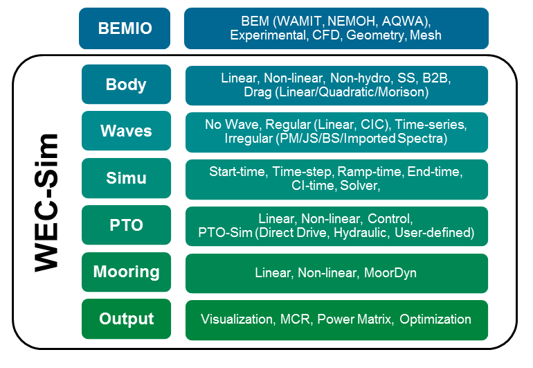
The diagram below highlights some of WEC-Sim’s advanced features, details of
which will be described in the following sections. Most advanced features have
a corresponding example case within the WEC-Sim_Applications repository or the WEC-Sim/Examples
directory in the WEC-Sim source code. For those topics of interest, it is
recommended that users run and understand the output of an application while
reading the documentation on the feature.
BEMIO
The Boundary Element Method Input/Output (BEMIO) functions are used to pre-process the BEM hydrodynamic data prior to running WEC-Sim. For more information about the WEC-Sim workflow, refer to Running WEC-Sim. The following section can also be followed in conjunction with the cases in the WEC-Sim/Examples directory in the WEC-Sim source code. This includes several cases with WAMIT, NEMOH, Aqwa, and Capytaine. For more information, refer to Series 1 - Multiple Condition Runs (MCR). BEMIO functions perform the following tasks:
Read BEM results from WAMIT, NEMOH, Aqwa, or Capytaine.
Calculate the radiation and excitation impulse response functions (IRFs).
Calculate the state space realization for the radiation IRF.
Save the resulting data in Hierarchical Data Format 5 (HDF5).
Plot typical hydrodynamic data for user verification.
Note
Previously the python based BEMIO code was used for this purpose. The python BEMIO functions have been converted to MATLAB and are included in the WEC-Sim source code. The python based BEMIO code will remain available but will no longer be supported.
BEMIO Functions
- functions.BEMIO.readWAMIT(hydro, filename, exCoeff)
Reads data from a WAMIT output file.
If generalized body modes are used, the output directory must also include the *.cfg, *.mmx, and *.hst files. If simu.nonlinearHydro = 3 will be used, the output directory must also include the *.3fk and *.3sc files.
See
WEC-Sim/examples/BEMIO/WAMITfor examples of usage.- Parameters:
hydro (
struct) – Structure of hydro data that WAMIT input data will be appended tofilename (
string) – Path to the WAMIT output fileexCoeff (
integer) – Flag indicating the type of excitation force coefficients to read, ‘diffraction’ (default), ‘haskind’, or ‘rao’
- Returns:
hydro – Structure of hydro data with WAMIT data appended
- Return type:
struct
- functions.BEMIO.readNEMOH(hydro, filedir)
Reads data from a NEMOH working folder.
See
WEC-Sim\examples\BEMIO\NEMOHfor examples of usage.- Parameters:
hydro (
struct) – Structure of hydro data that NEMOH input data will be appended tofilename (
string) –Path to the NEMOH working folder, must include:
Nemoh.calMesh/Hydrostatics.dat(orHydrostatiscs_0.dat,Hydrostatics_1.dat, etc. for multiple bodies)Mesh/KH.dat (or ``KH_0.dat,KH_1.dat, etc. for multiple bodies)Results/RadiationCoefficients.tecResults/ExcitationForce.tecResults/DiffractionForce.tec- If simu.nonlinearHydro = 3 will be usedResults/FKForce.tec- If simu.nonlinearHydro = 3 will be used
- Returns:
hydro – Structure of hydro data with NEMOH data appended
- Return type:
struct
Note
Instructions on how to download and use the open source BEM code NEMOH are provided on the NEMOH website.
The NEMOH Mesh.exe code creates the
Hydrostatics.datandKH.datfiles (among other files) for one input body at a time. For the readNEMOH function to work correctly in the case of a multiple body system, the user must manually renameHydrostatics.datandKH.datfiles toHydrostatics_0.dat,Hydrostatics_1.dat, …, andKH_0.dat,KH_1.dat,…, corresponding to the body order specified in theNemoh.calfile.
- functions.BEMIO.readAQWA(hydro, ah1Filename, lisFilename)
Reads data from AQWA output files.
See
WEC-Sim\examples\BEMIO\AQWAfor examples of usage.- Parameters:
hydro (
struct) – Structure of hydro data that Aqwa input data will be appended toah1Filename (
string) – .AH1 AQWA output filelisFilename (
string) – .LIS AQWA output file
- Returns:
hydro – Structure of hydro data with Aqwa data appended
- Return type:
struct
- functions.BEMIO.readCAPYTAINE(hydro, filename, hydrostatics_sub_dir)
Reads data from a Capytaine netcdf file
See
WEC-Sim\examples\BEMIO\CAPYTAINEfor examples of usage.- Parameters:
hydro (
struct) – Structure of hydro data that Capytaine input data will be appended tofilename (
string) – Capytaine .nc output filehydrostatics_sub_dir (
string) – Path to directory where Hydrostatics.dat and KH.dat files are saved
- Returns:
hydro – Structure of hydro data with Capytaine data appended
- Return type:
struct
- functions.BEMIO.normalizeBEM(hydro)
Normalizes BEM hydrodynamic coefficients in the same manner that WAMIT outputs are normalized. Specifically, the linear restoring stiffness is normalized as \(C_{i,j}/(\rho g)\); added mass is normalized as \(A_{i,j}/\rho\); radiation damping is normalized as \(B_{i,j}/(\rho \omega)\); and, exciting forces are normalized as \(X_i/(\rho g)\). And, if necessary, sort data according to ascending frequency.
This function is not called directly by the user; it is automatically implemented within the readWAMIT, readCAPYTAINE, readNEMOH, and readAQWA functions.
- Parameters:
hydro (
[1 x 1] struct) – Structure of hydro data that will be normalized and sorted depending on the value of hydro.code- Returns:
hydro – Normalized hydro data
- Return type:
[1 x 1] struct
- functions.BEMIO.combineBEM(hydro)
Combines multiple BEM outputs into one hydrodynamic ‘system.’ This function requires that all BEM outputs have the same water depth, wave frequencies, and wave headings. This function would be implemented following multiple readWAMIT, readNEMOH, readCAPYTAINE, or readAQWA and before radiationIRF, radiationIRFSS, excitationIRF, writeBEMIOH5, or plotBEMIO function calls.
See
WEC-Sim\examples\BEMIO\NEMOHfor examples of usage.- Parameters:
hydro (
[1 x n] struct) – Structures of hydro data that will be combined into a single structure- Returns:
hydro – Combined structure.
- Return type:
[1 x 1] struct
- functions.BEMIO.radiationIRF(hydro, tEnd, nDt, nDw, wMin, wMax)
Calculates the normalized radiation impulse response function. This is equivalent to the radiation IRF in the theory section normalized by \(\rho\):
\(\overline{K}_{r,i,j}(t) = {\frac{2}{\pi}}\intop_0^{\infty}{\frac{B_{i,j}(\omega)}{\rho}}\cos({\omega}t)d\omega\)
Default parameters can be used by inputting []. See
WEC-Sim\examples\BEMIOfor examples of usage.- Parameters:
hydro (
struct) – Structure of hydro datatEnd (
float) – Calculation range for the IRF, where the IRF is calculated from t = 0 to tEnd, and the default is 100 snDt (
float) – Number of time steps in the IRF, the default is 1001nDw (
float) – Number of frequency steps used in the IRF calculation (hydrodynamic coefficients are interpolated to correspond), the default is 1001wMin (
float) – Minimum frequency to use in the IRF calculation, the default is the minimum frequency from the BEM datawMax (
float) – Maximum frequency to use in the IRF calculation, the default is the maximum frequency from the BEM data
- Returns:
hydro – Structure of hydro data with radiation IRF
- Return type:
struct
- functions.BEMIO.radiationIRFSS(hydro, Omax, R2t)
Calculates the state space (SS) realization of the normalized radiation IRF. If this function is used, it must be implemented after the radiationIRF function.
Default parameters can be used by inputting []. See
WEC-Sim\examples\BEMIOfor examples of usage.- Parameters:
hydro (
struct) – Structure of hydro dataOmax (
integer) – Maximum order of the SS realization, the default is 10R2t (
float) – \(R^2\) threshold (coefficient of determination) for the SS realization, where \(R^2\) may range from 0 to 1, and the default is 0.95
- Returns:
hydro – Structure of hydro data with radiation IRF state space coefficients
- Return type:
struct
- functions.BEMIO.excitationIRF(hydro, tEnd, nDt, nDw, wMin, wMax)
Calculates the normalized excitation impulse response function:
\(\overline{K}_{e,i,\theta}(t) = {\frac{1}{2\pi}}\intop_{-\infty}^{\infty}{\frac{X_i(\omega,\theta)e^{i{\omega}t}}{{\rho}g}}d\omega\)
Default parameters can be used by inputting []. See
WEC-Sim\examples\BEMIOfor examples of usage.- Parameters:
hydro (
struct) – Structure of hydro datatEnd (
float) – Calculation range for the IRF, where the IRF is calculated from t = 0 to tEnd, and the default is 100 snDt (
float) – Number of time steps in the IRF, the default is 1001nDw (
float) – Number of frequency steps used in the IRF calculation (hydrodynamic coefficients are interpolated to correspond), the default is 1001wMin (
float) – Minimum frequency to use in the IRF calculation, the default is the minimum frequency from the BEM datawMax (
float) – Maximum frequency to use in the IRF calculation, the default is the maximum frequency from the BEM data
- Returns:
hydro – Structure of hydro data with excitation IRF
- Return type:
struct
- functions.BEMIO.readBEMIOH5(filename, number, meanDrift)
Function to read BEMIO data from an h5 file into a hydrodata structure for the bodyClass
- Parameters:
filename (
string) – Path to the BEMIO .h5 file to readnumber (
integer) – Body number to read from the .h5 file. For example, body(2) in the input file must read body2 from the .h5 file.meanDrift (
integer) – Flag to optionally read mean drift force coefficients
- Returns:
hydroData – Struct of hydroData used by the bodyClass. Different format than the BEMIO hydro struct
- Return type:
struct
- functions.BEMIO.reverseDimensionOrder(inputData)
This function reverse the order of the dimensions in data. Called by readBEMIOH5() to permute data into the correct format.
This required permutation is a legacy of the
Load_H5function that reordered dimensions of hydroData after reading- Parameters:
inputData (
array) – Any numeric data array- Returns:
outputData – Input data array with the order of its dimensions reversed
- Return type:
array
- functions.BEMIO.calcSpectralMoment(angFreq, S_f, order)
- Parameters:
angFreq (
[1 n] float vector) – Vector of wave angular frequenciesS_f (
[1 n] float vector) – Vector of wave spectraorder (
float) – Order of the spectral moment
- Returns:
mn – Spectral moment of the nth order
- Return type:
float vector
- functions.BEMIO.calcWaveNumber(omega, waterDepth, g, deepWater)
Solves the wave dispersion relation \(\omega^2 = g k*tanh(k h)\) for the wave number
- Parameters:
omega (
float) – Wave frequency [rad/s]waterDepth (
float) – Water depth [m]g (
float) – Gravitational acceleration [m/s^2]deepWater (
integar) – waveClass flag inidicating a deep water wave [-]
- Returns:
k – Wave number [m]
- Return type:
float
- functions.BEMIO.writeBEMIOH5(hydro)
Writes the hydro data structure to a .h5 file.
See
WEC-Sim\tutorials\BEMIOfor examples of usage.- Parameters:
hydro (
[1 x 1] struct) – Structure of hydro data that is written tohydro.file
Note
Technically, this step should not be necessary - the MATLAB data structure hydro is written to a *.h5 file by BEMIO and then read back into a new MATLAB data structure hydroData for each body by WEC-Sim. The reasons this step was retained were, first, to remain compatible with the python based BEMIO output and, second, for the simpler data visualization and verification capabilities offered by the *.h5 file viewer.
- functions.BEMIO.plotBEMIO(varargin)
Plots the added mass, radiation damping, radiation IRF, excitation force magnitude, excitation force phase, and excitation IRF for each body in the given degrees of freedom.
Usage:
plotBEMIO(hydro, hydro2, hydro3, ...)See
WEC-Sim\examples\BEMIOfor additional examples.- Parameters:
varargin (
struct(s)) – The hydroData structure(s) created by the other BEMIO functions. One or more may be input.
- functions.BEMIO.plotAddedMass(varargin)
Plots the added mass for each hydro structure’s bodies in the given degrees of freedom.
Usage:
plotAddedMass(hydro, hydro2, hydro3, ...)- Parameters:
varargin (
struct(s)) – The hydroData structure(s) created by the other BEMIO functions. One or more may be input.
- functions.BEMIO.plotRadiationDamping(varargin)
Plots the radiation damping for each hydro structure’s bodies in the given degrees of freedom.
Usage:
plotRadiationDamping(hydro, hydro2, hydro3, ...)- Parameters:
varargin (
struct(s)) – The hydroData structure(s) created by the other BEMIO functions. One or more may be input.
- functions.BEMIO.plotRadiationIRF(varargin)
Plots the radiation IRF for each hydro structure’s bodies in the given degrees of freedom.
Usage:
plotRadiationIRF(hydro, hydro2, hydro3, ...)- Parameters:
varargin (
struct(s)) – The hydroData structure(s) created by the other BEMIO functions. One or more may be input.
- functions.BEMIO.plotExcitationMagnitude(varargin)
Plots the excitation force magnitude for each hydro structure’s bodies in the given degrees of freedom.
Usage:
plotExcitationMagnitude(hydro, hydro2, hydro3, ...)- Parameters:
varargin (
struct(s)) – The hydroData structure(s) created by the other BEMIO functions. One or more may be input.
- functions.BEMIO.plotExcitationPhase(varargin)
Plots the excitation force phase for each hydro structure’s bodies in the given degrees of freedom.
Usage:
plotExcitationPhase(hydro, hydro2, hydro3, ...)- Parameters:
varargin (
struct(s)) – The hydroData structure(s) created by the other BEMIO functions. One or more may be input.
- functions.BEMIO.plotExcitationIRF(varargin)
Plots the excitation IRF for each hydro structure’s bodies in the given degrees of freedom.
Usage:
plotExcitationIRF(hydro, hydro2, hydro3, ...)- Parameters:
varargin (
struct(s)) – The hydroData structure(s) created by the other BEMIO functions. One or more may be input.
BEMIO hydro Data Structure
Variable |
Format |
Description |
A |
[nDOF,nDOF,Nf] |
radiation added mass |
Ainf |
[nDOF,nDOF] |
infinite frequency added mass |
B |
[nDOF,nDOF,Nf] |
radiation wave damping |
theta |
[1,Nh] |
wave headings (deg) |
body |
{1,Nb} |
body names |
cb |
[3,Nb] |
center of buoyancy |
cg |
[3,Nb] |
center of gravity |
code |
string |
BEM code (WAMIT, NEMOH, AQWA, or CAPYTAINE) |
K_hs |
[6,6,Nb] |
hydrostatic restoring stiffness |
dof |
[1, Nb] |
Degrees of freedom (DOF) for each body. Default DOF for each body is 6 plus number of possible generalized body modes (GBM). |
ex_im |
[nDOF,Nh,Nf] |
imaginary component of excitation force or torque |
ex_K |
[nDOF,Nh,length(ex_t)] |
excitation IRF |
ex_ma |
[nDOF,Nh,Nf] |
magnitude of excitation force or torque |
ex_ph |
[nDOF,Nh,Nf] |
phase of excitation force or torque |
ex_re |
[nDOF,Nh,Nf] |
real component of excitation force or torque |
ex_t |
[1,length(ex_t)] |
time steps in the excitation IRF |
ex_w |
[1,length(ex_w)] |
frequency step in the excitation IRF |
file |
string |
BEM output filename |
fk_im |
[nDOF,Nh,Nf] |
imaginary component of Froude-Krylov contribution to the excitation force or torque |
fk_ma |
[nDOF,Nh,Nf] |
magnitude of Froude-Krylov excitation component |
fk_ph |
[nDOF,Nh,Nf] |
phase of Froude-Krylov excitation component |
fk_re |
[nDOF,Nh,Nf] |
real component of Froude-Krylov contribution to the excitation force or torque |
g |
[1,1] |
gravity |
h |
[1,1] |
water depth |
Nb |
[1,1] |
number of bodies |
Nf |
[1,1] |
number of wave frequencies |
Nh |
[1,1] |
number of wave headings |
plotDofs |
[length(plotDofs),2] |
degrees of freedom to be plotted (default: [1,1;3,3;5,5]) |
plotBodies |
[1,length(plotBodies)] |
BEM bodies to be plotted (default: [1:Nb]) |
plotDirections |
[1,length(plotDirections)] |
indices indicating wave directions to plot from list of headings (default: [1]) |
ra_K |
[nDOF,nDOF,length(ra_t)] |
radiation IRF |
ra_t |
[1,length(ra_t)] |
time steps in the radiation IRF |
ra_w |
[1,length(ra_w)] |
frequency steps in the radiation IRF |
rho |
[1,1] |
density |
sc_im |
[nDOF,Nh,Nf] |
imaginary component of scattering contribution to the excitation force or torque |
sc_ma |
[nDOF,Nh,Nf] |
magnitude of scattering excitation component |
sc_ph |
[nDOF,Nh,Nf] |
phase of scattering excitation component |
sc_re |
[nDOF,Nh,Nf] |
real component of scattering contribution to the excitation force or torque |
ss_A |
[nDOF,nDOF,ss_O,ss_O] |
state space A matrix |
ss_B |
[nDOF,nDOF,ss_O,1] |
state space B matrix |
ss_C |
[nDOF,nDOF,1,ss_O] |
state space C matrix |
ss_conv |
[nDOF,nDOF] |
state space convergence flag |
ss_D |
[nDOF,nDOF,1] |
state space D matrix |
ss_K |
[nDOF,nDOF,length(ra_t)] |
state space radiation IRF |
ss_O |
[nDOF,nDOF] |
state space order |
ss_R2 |
[nDOF,nDOF] |
state space R2 fit |
T |
[1,Nf] |
wave periods |
Vo |
[1,Nb] |
displaced volume |
w |
[1,Nf] |
wave frequencies |
Writing Your Own h5 File
The most common way of creating a *.h5 file is using BEMIO to post-process the outputs of a BEM code.
This requires a single BEM solution that contains all hydrodynamic bodies and accounts for body-to-body interactions.
Some cases in which you might want to create your own h5 file are:
Use experimentally determined coefficients or a mix of BEM and experimental coefficients.
Combine results from different BEM files and have the coefficient matrices be the correct size for the new total number of bodies.
Modify the BEM results for any other reason.
MATLAB and Python have functions to read and write *.h5 files easily.
WEC-Sim includes one function writeBEMIOH5 to help you create your own *.h5 file.
The first step is to have all the required coefficients and properties in Matlab in the correct hydroData format.
Then writeBEMIOH5 is used to create and populate the *.h5 file.
Simulation Features
This section provides an overview of WEC-Sim’s simulation class features; for more information about the simulation class code structure, refer to Simulation Class.
Running WEC-Sim
The subsection describes the various ways to run WEC-Sim. The standard method is
to type the command wecSim in the MATLAB command window when in a $CASE
directory. This is the same method described in the Workflow and
Tutorials sections.
Running as Function
WEC-Sim allows users to execute WEC-Sim as a function by using wecSimFcn.
This option may be useful for users who wish to devise their own batch runs,
isolate the WEC-Sim workspace, create a special set-up before running WEC-Sim,
or link to another software.
Running from Simulink
WEC-Sim can also be run directly from Simulink with the following steps:
Type
initializeWecSimin the Command WindowRun the model from Simulink and wait for the simulation to complete
Type
stopWecSimin the Command Window
This allows users to initialize WEC-Sim from the command window and then start the simulation from Simulink, allowing for greater compatibility with other models or hardware-in-the-loop simulations.
Multiple Condition Runs (MCR)
WEC-Sim allows users to easily perform batch runs by typing wecSimMCR into
the MATLAB Command Window. This command executes the Multiple Condition Run
(MCR) option, which can be initiated three different ways:
Option 1. Specify a range of sea states and PTO damping coefficients in the WEC-Sim input file, example:
waves.height = 1:0.5:5; waves.period = 5:1:15;pto(1).stiffness=1000:1000:10000; pto(1).damping=1200000:1200000:3600000;Option 2. Specify the excel filename that contains a set of wave statistic data in the WEC-Sim input file. This option is generally useful for power matrix generation, example:
simu.mcrExcelFile = "<Excel file name>.xls"Option 3. Provide a MCR case .mat file, and specify the filename in the WEC-Sim input file, example:
simu.mcrMatFile = "<File name>.mat"
For Multiple Condition Runs, the *.h5 hydrodynamic data is only loaded
once. To reload the *.h5 data between runs, set simu.reloadH5Data =1 in
the WEC-Sim input file.
If the Simulink model relies upon From Workspace input blocks other than those utilized by the WEC-Sim library blocks (e.g. waves.elevationFile), these can be iterated through using Option 3. The MCR file header MUST be a cell containing the exact string 'LoadFile'. The pathways of the files to be loaded to the workspace must be given in the cases field of the MCR .mat file. WEC-Sim MCR will then run WEC-Sim in sequence, once for each file to be loaded. The variable name of each loaded file should be consistent, and specified by the From Workspace block.
For more information, refer to Series 1 - Multiple Condition Runs (MCR), and the RM3_MCR example on the WEC-Sim Applications repository.
The RM3_MCR examples on the WEC-Sim Applications repository demonstrate the use of WEC-Sim MCR for each option above (arrays, .xls, .mat). The fourth case demonstrates how to vary the wave spectrum input file in each case run by WEC-Sim MCR.
The directory of an MCR case can contain a userDefinedFunctionsMCR.m
file that will function as the standard userDefinedFunctions.m file.
Within the MCR application, the userDefinedFunctionsMCR.m script
creates a power matrix from the PTO damping coefficient after all cases have
been run.
For more information, refer to Series 1 - Multiple Condition Runs (MCR).
Parallel Computing Toolbox (PCT)
WEC-Sim allows users to execute batch runs by typing wecSimPCT into the
MATLAB Command Window. This command executes the MATLAB Parallel Computing
Toolbox (PCT),
which allows parallel capability for Multiple Condition Runs (MCR) but adds
an additional MATLAB dependency to use this feature. Similar to MCR, this
feature can be executed in three ways (Options 1~3).
For PCT runs, the *.h5 hydrodynamic data must be reloaded, regardless the
setting for simu.reloadH5Data in the WEC-Sim input file.
The option simu.keepPool=1 will retain the parallel pool after simulations have finished to facilitate
parallel post-processing. If the pool is no longer needed or needs reinitialization, simu.keepPool=0 will close the parallel pool after simulations have completed.
Note
The userDefinedFunctionsMCR.m is not compatible with wecSimPCT.
Please use userDefinedFunctions.m instead.
Radiation Force calculation
The radiation forces are calculated at each time-step by the convolution of the body velocity and the radiation Impulse Response Function – which is calculated using the cosine transform of the radiation-damping. Speed-gains to the simulation can be made by using alternatives to the convolution operation, namely,
The State-Space Representation,
The Finite Impulse Response (FIR) Filters.
Simulation run-times were benchmarked using the RM3 example simulated for 1000 s. Here is a summary of normalized run-times when the radiation forces are calculated using different routes. The run-times are normalized by the run-time for a simulation where the radiation forces are calculated using “Constant Coefficients” ( \(T_0\) ):
Radiation Force Calculation Approach
Normalized Run Time
Constant Coefficients
\(T_0\)
Convolution
\(1.57 \times T_0\)
State-Space
\(1.14 \times T_0\)
FIR Filter
\(1.35 \times T_0\)
State-Space Representation
The convolution integral term in the equation of motion can be linearized using
the state-space representation as described in the Theory Manual section. To
use a state-space representation, the simu.stateSpace simulationClass variable
must be defined in the WEC-Sim input file, for example:
simu.stateSpace = 1
Finite Impulse Response (FIR) Filters
By default, WEC-Sim uses numerical integration to calculate the convolution integral, while FIR filters implement the same using a discretized convolution, by using FIR filters – digital filters that are inherently stable. Convolution of Impulse Response Functions of Finite length, i.e., those that dissipate and converge to zero can be accomplished using FIR filters. The convolution integral can also be calculated using FIR filters by setting:
simu.FIR=1.
Note
By default simu.FIR=0, unless specified otherwise.
Time-Step Features
The default WEC-Sim solver is ‘ode4’. Refer to the NonlinearHydro example on the WEC-Sim Applications repository for a comparisons between ‘ode4’ to ‘ode45’. The following variables may be changed in the simulationClass (where N is number of increment steps, default: N=1):
Fixed time-step:
simu.dtOutput time-step:
simu.dtOut=N*simu.dtNonlinear Buoyancy and Froude-Krylov Excitation time-step:
simu.nonlinearDt=N*simu.dtConvolution integral time-step:
simu.cicDt=N*simu.dtMorison force time-step:
simu.morisonDt = N*simu.dt
Fixed Time-Step (ode4)
When running WEC-Sim with a fixed time-step, 100-200 time-steps per wave period is recommended to provide accurate hydrodynamic force calculations (ex: simu.dt = T/100, where T is wave period). However, a smaller time-step may be required (such as when coupling WEC-Sim with MoorDyn or PTO-Sim). To reduce the required WEC-Sim simulation time, a different time-step may be specified for nonlinear buoyancy and Froude-Krylov excitation and for convolution integral calculations. For all simulations, the time-step should be chosen based on numerical stability and a convergence study should be performed.
Variable Time-Step (ode45)
To run WEC-Sim with a variable time-step, the following variables must be defined in the simulationClass:
Numerical solver:
simu.solver='ode45'Max time-step:
simu.dt
This option sets the maximum time step of the simulation (simu.dt) and
automatically adjusts the instantaneous time step to that required by MATLAB’s
differential equation solver.
Wave Features
This section provides an overview of WEC-Sim’s wave class features. For more
information about the wave class code structure, refer to
Wave Class. The various wave features can be
compared by running the cases within the WEC-Sim/Examples/RM3 and the
WEC-Sim/Examples/OSWEC directories.
Irregular Wave Binning
WEC-Sim’s default spectral binning method divides the wave spectrum into 499 bins with equal energy content, defined by 500 wave frequencies. As a result, the wave forces on the WEC using the equal energy method are only computed at each of the 500 wave frequencies. The equal energy formulation speeds up the irregular wave simulation time by reducing the number of frequencies the wave train is defined by, and thus the number of frequencies for which the wave forces are calculated. It prevents bins with very little energy from being created and unnecessarily adding to the computational cost. The equal energy method is specified by defining the following wave class variable in the WEC-Sim input file:
waves.bem.option = 'EqualEnergy';
By comparison, the traditional method divides the wave spectrum into a sufficiently large number of equally spaced bins to define the wave spectrum. WEC-Sim’s traditional formulation uses 999 bins, defined by 1000 wave frequencies of equal frequency distribution. To override WEC-Sim’s default equal energy method, and instead use the traditional binning method, the following wave class variable must be defined in the WEC-Sim input file:
waves.bem.option = 'Traditional';
Users may override the default number of wave frequencies by defining
waves.bem.count. However, it is on the user to ensure that the wave spectrum
is adequately defined by the number of wave frequencies, and that the wave
forces are not impacted by this change.
Wave Directionality
WEC-Sim has the ability to model waves with various angles of incidence, \(\theta\). To define wave directionality in WEC-Sim, the following wave class variable must be defined in the WEC-Sim input file:
waves.direction = <user defined wave direction(s)>; %[deg]
The incident wave direction has a default heading of 0 Degrees (Default = 0), and should be defined as a column vector for more than one wave direction. For more information about the wave formulation, refer to Wave Spectra.
Wave Directional Spreading
WEC-Sim has the ability to model waves with directional spreading, \(D\left( \theta \right)\). To define wave directional spreading in WEC-Sim, the following wave class variable must be defined in the WEC-Sim input file:
waves.spread = <user defined directional spreading>;
The wave directional spreading has a default value of 1 (Default = 1), and should be defined as a column vector of directional spreading for each one wave direction. For more information about the spectral formulation, refer to Wave Spectra.
Note
Users must define appropriate spreading parameters to ensure energy is conserved. Recommended directional spreading functions include Cosine-Squared and Cosine-2s.
For full-directional waves, the spreading is defined differently (does not sum to 1) and the parameter waves.fullDirectionalSpectrum.spread is used in place of waves.spread. Refer to spectrumImportFullDir for more information.
Multiple Wave-Spectra
The Wave Directional Spreading feature only allows splitting the same wave-front. However, quite often mixed-seas are composed of disparate Wave-Spectra with unique periods, heights, and directions. An example would be a sea-state composed of swell-waves and chop-waves.
Assuming that the linear potential flow theory holds, the wave inputs to the system can be super-imposed. This implies, the effects of multiple Wave-Spectra can be simulated, if the excitation-forces for each Wave-Spectra is calculated, and added to the pertinent Degree-of-Freedom.
WEC-Sim can simulate the dynamics of a body experiencing multiple Wave-Spectra each with
their unique directions, periods, and heights. In order to calculate the excitation-forces
for multiple Wave-Spectra, WEC-Sim automatically generates multiple instances of
excitation-force sub-systems. The user only needs to create multiple instances of
the waves class.
Here is an example for setting up multiple Wave-Spectra in the WEC-Sim input file:
waves(1)           = waveClass('regularCIC');   % Initialize Wave Class and Specify Type
waves(1).height    = 2.5;                       % Wave Height [m]
waves(1).period    = 8;                         % Wave Period [s]
waves(1).direction = 0;                         % Wave Direction (deg.)
waves(2)           = waveClass('regularCIC');   % Initialize Wave Class and Specify Type
waves(2).height    = 2.5;                       % Wave Height [m]
waves(2).period    = 8;                         % Wave Period [s]
waves(2).direction = 90;                        % Wave Direction (deg.)
Note
1. If using a wave-spectra with different wave-heading directions, ensure that the BEM data has the hydrodynamic coefficients corresponding to the desired wave-heading direction,
2. All wave-spectra should be of the same type, i.e., if waves(1) is initialized
as waves(1) = waveClass('regularCIC'), the following waves(#) object should
initialized the same way.
Addtionally, the multiple Wave-Spectra can be visualized as elaborated in Wave Markers. The user needs to define the marker parameters for each Wave-Spectra, as one would for a single Wave-Spectra.
Here is an example of 2 Wave-Spectra being visualized using the wave wave-markers feature:
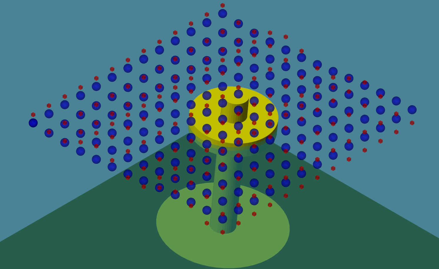
Here is a visualization of two Wave-Spectra, represented by red markers and blue markers respectively.
Irregular Waves with Seeded Phase
By default, the phase for all irregular wave cases are generated randomly. In order to reproduce the same time-series every time an irregular wave simulation is run, the following wave class variable may be defined in the WEC-Sim input file:
waves.phaseSeed = <user defined seed>;
By setting waves.phaseSeed equal to 1,2,3,…,etc, the random wave phase
generated by WEC-Sim is seeded, thus producing the same random phase for each
simulation.
Wave Gauge Placement
Wave gauges can be included through the wave class parameters:
waves.marker.location
waves.marker.size
waves.marker.style
By default, the wave surface elevation at the origin is calculated by WEC-Sim. In past releases, there was the option to define up to three numerical wave gauge locations where WEC-Sim would also calculate the undisturbed linear incident wave elevation. WEC-Sim now has the feature to define wave markers that oscillate vertically with the undistrubed linear wave elevation (see Wave Markers). This feature does not limit the number of point measurements of the undisturbed free surface elevation and the time history calculation at the marker location is identical to the previous wave gauge implementation. Users who desire to continuing using the previous wave gauge feature will only need to update the variable called within WEC-Sim and an example can be found in the WECCCOMP Repository.
Note
The numerical wave markers (wave gauges) do not handle the incident wave interaction with the radiated or diffracted waves that are generated because of the presence and motion of any hydrodynamic bodies.
Ocean Current
The speed of an ocean current can be included through the wave class parameters:
waves.current.option
waves.current.speed
waves.current.direction
waves.current.depth
The current option determines the method used to propagate the surface current across the
specified depth. Option 0 is depth independent, option 1 uses a 1/7 power law, option 2
uses linear variation with depth and option 3 specifies no ocean current.
The current.speed parameter represents the surface current speed, and current.depth
the depth at which the current speed decays to zero (given as a positive number).
See Ocean Current for more details on each method.
These parameters are used to calculate the fluid velocity in the Morison Element calculation.
Body Features
This section provides an overview of WEC-Sim’s body class features; for more information about the body class code structure, refer to Body Class.
Body Mass and Geometry Features
The mass of each body must be specified in the WEC-Sim input file. The following features are available:
Floating Body - the user may set
body(i).mass = 'equilibrium'which will calculate the body mass based on displaced volume and water density. Ifsimu.nonlinearHydro = 0, then the mass is calculated using the displaced volume contained in the*.h5file. Ifsimu.nonlinearHydro = 1orsimu.nonlinearHydro = 2, then the mass is calculated using the displaced volume of the provided STL geometry file.Fixed Body - if a body is fixed to the seabed using a fixed constraint, the mass and moment of inertia may be set to arbitrary values such as 999 kg and [999 999 999] kg-m^2. If the constraint forces on the fixed body are important, the mass and inertia should be set to their real values.
Import STL - to read in the geometry (
*.stl) into Matlab use thebody(i).importBodyGeometry()method in the bodyClass. This method will import the mesh details (vertices, faces, normals, areas, centroids) into thebody(i).geometryproperty. This method is also used for nonlinear buoyancy and Froude-Krylov excitation and ParaView visualization files. Users can then visualize the geometry using thebody(i).plotStlmethod.
Nonlinear Buoyancy and Froude-Krylov Excitation
WEC-Sim has the option to include the nonlinear hydrostatic restoring and Froude-Krylov forces when solving the system dynamics of WECs, accounting for the weakly nonlinear effect on the body hydrodynamics. To use nonlinear buoyancy and Froude-Krylov excitation, the body(ii).nonlinearHydro bodyClass variable must be defined in the WEC-Sim input file, for example:
body(ii).nonlinearHydro = 2
For more information, refer to the Series 2 - Nonlinear Buoyancy and Froude-Krylov Wave Excitation, and the NonlinearHydro example on the WEC-Sim Applications repository.
Nonlinear Settings
body(ii).nonlinearHydro -
The nonlinear hydrodynamics option can be used with the parameter:
body(ii).nonlinearHydro in your WEC-Sim input file. When any of the three
nonlinear options (below) are used, WEC-Sim integrates the wave pressure over
the surface of the body, resulting in more accurate buoyancy and Froude-Krylov
force calculations.
Option 1.
body(ii).nonlinearHydro = 1This option integrates the pressure due to the mean wave elevation and the instantaneous body position.Option 2.
body(ii).nonlinearHydro = 2This option integrates the pressure due to the instantaneous wave elevation and the instantaneous body position. This option is recommended if nonlinear effects need to be considered.
simu.nonlinearDt -
An option available to reduce the nonlinear simulation time is to specify a
nonlinear time step, simu.nonlinearDt=N*simu.dt, where N is number of
increment steps. The nonlinear time step specifies the interval at which the
nonlinear hydrodynamic forces are calculated. As the ratio of the nonlinear to
system time step increases, the computation time is reduced, again, at the
expense of the simulation accuracy.
Note
WEC-Sim’s nonlinear buoyancy and Froude-Krylov wave excitation option may be used for regular or irregular waves but not with user-defined irregular waves.
STL File Generation
When the nonlinear option is turned on, the geometry file (*.stl)
(previously only used for visualization purposes in linear simulations) is used
as the discretized body surface on which the nonlinear pressure forces are
integrated. As in the linear case, the STL mesh origin must be at a body’s center of gravity.
A good STL mesh resolution is required when using the nonlinear buoyancy and Froude-Krylov wave excitation in
WEC-Sim. The simulation accuracy will increase with increased surface
resolution (i.e. the number of discretized surface panels specified in the
*.stl file), but the computation time will also increase.
There are many ways to generate an STL file; however, it is important to verify
the quality of the mesh before running WEC-Sim simulations with the nonlinear
hydro flag turned on. An STL file can be exported from most CAD programs, but
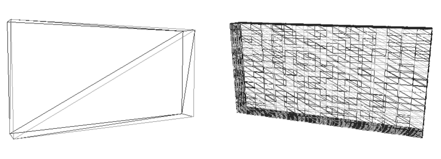
few allow adequate mesh refinement. By default, most CAD programs write an STL
file similar to the left figure, with the minimum panels possible.
To accurately model nonlinear hydrodynamics in WEC-Sim, STL files should be refined to
have an aspect ratio close to one, and contain a high resolution in the vertical direction
so that an accurate instantaneous displaced volume can be calculated.
Many commercial and free software exist to convert between mesh formats and refine STL files, including:
Coreform CUBIT (commercial)
Rhino (commercial)
Nonlinear Buoyancy and Froude-Krylov Wave Excitation Tutorial - Heaving Ellipsoid
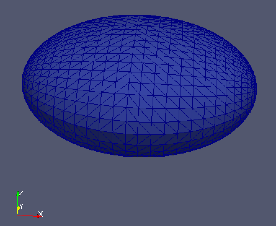
The body tested in the study is an ellipsoid with a cross- section characterized by semi-major and -minor axes of 5.0 m and 2.5 m in the wave propagation and normal directions, respectively . The ellipsoid is at its equilibrium position with its origin located at the mean water surface. The mass of the body is then set to 1.342×10⁵ kg, and the center of gravity is located 2 m below the origin.
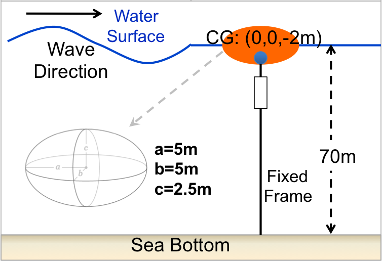
STL file with the discretized body surface is shown below (ellipsoid.stl)
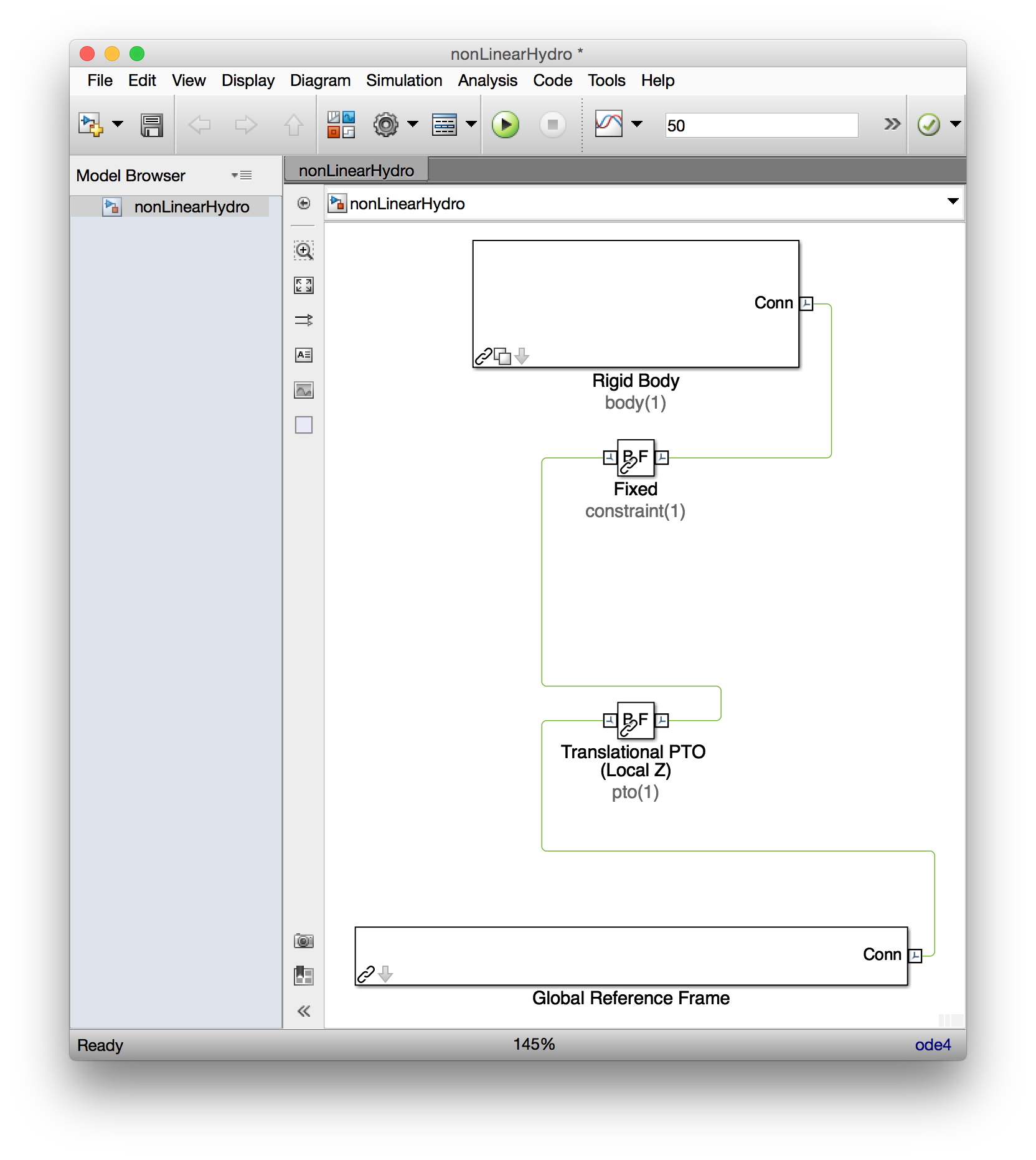
The single-body heave only WEC model is shown below (nonLinearHydro.slx)
The WEC-Sim input file used to run the nonlinear hydro WEC-Sim simulation:
%% Simulation Data
simu = simulationClass();
simu.simMechanicsFile = 'ellipsoid.slx';
simu.mode = 'normal';                   % Specify Simulation Mode ('normal','accelerator','rapid-accelerator')
simu.explorer='off';                     % Turn SimMechanics Explorer (on/off)
simu.startTime = 0;
simu.rampTime = 50;
simu.endTime=150;
simu.dt = 0.05;
simu.rho=1025;

%% Wave Information
% Regular Waves
waves = waveClass('regular');
waves.height = 4;
waves.period = 6;

%% Body Data
body(1) = bodyClass('../../hydroData/ellipsoid.h5');
body(1).mass = 'equilibrium';
body(1).inertia = ...
    [1.375264e6 1.375264e6 1.341721e6];
body(1).geometryFile = '../../geometry/elipsoid.stl' ;
body(1).quadDrag.cd=[1 0 1 0 1 0];
body(1).quadDrag.area=[25 0 pi*5^2 0 pi*5^5 0];
body(1).nonlinearHydro = 2;                       % Non-linear hydro on/off

%% PTO and Constraint Parameters
% Fixed Constraint
constraint(1) = constraintClass('Constraint1');
constraint(1).location = [0 0 -12.5];

% Translational PTO
pto(1) = ptoClass('PTO1');
pto(1).stiffness=0;
pto(1).damping=1200000;
pto(1).location = [0 0 -12.5];
Simulation and post-processing is the same process as described in the Tutorials section.
Viscous Damping and Morison Elements
WEC-Sim allows for the definition of additional damping and added-mass terms to allow users to tune their models precisely. Viscous damping and Morison Element may be defined for hydrodynamic, drag, or flexible bodies. It is highly recommended that users add viscous or Morison drag to create a realistic model.
When the Morison Element
option is used in combination with a hydrodynamic or flexible body, it serves as a
tuning method. The equation of motion for hydrodynamic and flexible bodies with a
Morison Element is more complex than the traditional Morison Element formulation.
A traditional Morison Element may be created by using a drag body
(body(#).nonHydro=2) with body(#).morisonElement.option = 1 or 2.
For more information about the numerical formulation of viscous damping and
Morison Elements, refer to the theory section Viscous Damping and Morison Elements.
Viscous Damping
A viscous damping force in the form of a linear damping coefficient \(C_{v}\) can be applied to each body by defining the following body class parameter in the WEC-Sim input file (which has a default value of zero):
body(i).linearDamping
A quadratic drag force, proportional to the square of the body’s velocity, can be applied to each body by defining the quadratic drag coefficient \(C_{d}\), and the characteristic area \(A_{d}\) for drag calculation. This is achieved by defining the following body class parameters in the WEC-Sim input file (each of which have a default value of zero):
body(i).quadDrag.cd
body(i).quadDrag.area
Alternatively, one can define \(C_{D}\) directly:
body(i).quadDrag.drag
Morison Elements
To use Morison Elements, the following body class variable must be
defined in the WEC-Sim input file with body(ii).morisonElement.option.
Implementation Option 0 Morison Elements are not included in the body force and moment calculations.
Implementation Option 1 allows for the Morison Element properties to be defined independently for the x-, y-, and z-axis while Implementation Option 2 uses a normal and tangential representation of the Morison Element properties. Note that the two options allow the user flexibility to implement hydrodynamic forcing that best suits their modeling needs; however, the two options have slightly different calculation methods and therefore the outputs will not necessarily provide the same forcing values. The user is directed to look at the Simulink Morison Element block within the WEC-Sim library to better determine which approach better suits their modeling requirements.
Morison Elements must be defined for each body using the
body(i).morisonElement property of the body class. This property
requires definition of the following body class parameters in the WEC-Sim input
file (each of which have a default value of zero(s)).
For body(ii).morisonElement.option = 1
body(i).morisonElement.cd = [c_{dx} c_{dy} c_{dz}]
body(i).morisonElement.ca = [c_{ax} c_{ay} c_{az}]
body(i).morisonElement.area = [A_{x} A_{y} A_{z}]
body(i).morisonElement.VME = [V_{me}]
body(i).morisonElement.rgME = [r_{gx} r_{gy} r_{gz}]
body(i).morisonElement.z = [0 0 0]
Note
For Option 1, the unit normal body(#).morisonElement.z must be
initialized as a [n x3] vector, where n is the number of Morison Elements, although it will not be used in the
hydrodynamic calculation.
For body(ii).morisonElement.option = 2
body(i).morisonElement.cd = [c_{dn} c_{dt} 0]
body(i).morisonElement.ca = [c_{an} c_{at} 0]
body(i).morisonElement.area = [A_{n} A_{t} 0]
body(i).morisonElement.VME = [V_{me}]
body(i).morisonElement.rgME = [r_{gx} r_{gy} r_{gz}]
body(i).morisonElement.z = [z_{x} z_{y} z_{z}]
Note
For Option 2, the body(i).morisonElement.cd,
body(i).morisonElement.ca, and
body(i).morisonElement.area variables need to be
initialized as [n x3] vector, where n is the number of Morison Elements, with the third column index set to zero. While
body(i).morisonElement.z is a unit normal vector that defines the
orientation of the Morison Element.
To better represent certain scenarios, an ocean current speed can be defined to
calculate a more accurate fluid velocity and acceleration on the Morison
Element. These can be defined through the wave class parameters
waves.current.option, waves.current.speed, waves.current.direction,
and waves.current.depth. See Ocean Current for more
detail on using these options.
The Morison Element time-step may also be defined as
simu.morisonDt = N*simu.dt, where N is number of increment steps. For an
example application of using Morison Elements in WEC-Sim, refer to the WEC-Sim
Applications repository
Free_Decay/1m-ME example.
Note
Morison Elements cannot be used with elevationImport.
Second-Order Excitation Forces and Quadratic Transfer Functions (QTFs)
For large offshore structures, second-order wave excitation forces can significantly influence system behavior—particularly in surge, pitch, and other low-frequency motions. These forces arise from interactions between pairs of wave frequencies, \(\omega_i\) and \(\omega_j\), within the wave spectrum.
There are two types of second-order forces:
Sum-frequency forces (\(\omega_i + \omega_j\)): High-frequency components that can excite fast body motions.
Difference-frequency forces (\(\omega_i - \omega_j\)): Low-frequency components that can induce slow-drift responses, commonly in surge or pitch.
WEC-Sim supports Quadratic Transfer Functions (QTFs) to model second-order excitation forces. These can be imported from hydrodynamic solvers such as WAMIT and NEMOH. BEMIO functions will automatically read, process, and write QTF coefficients from WAMIT and NEMOH to the *.h5 file.
File Naming and Conventions
The QTF file naming depends on the hydrodynamics solver:
WAMIT
QTF files should be located in the same folder as the .out file.
File naming format:
qtfResults_<body#>.11s
qtfResults_<body#>.11d
Example:
qtfWAMIT_1.11sNote: WAMIT uses 1-based indexing for body numbers.
NEMOH
QTF files should follow this naming format:
OUT_QTFP_N_<body#>.dat   (for sum-frequency QTFs)
OUT_QTFM_N_<body#>.dat   (for difference-frequency QTFs)
NEMOH uses 0-based indexing for body numbers.
Activating QTFs in WEC-Sim
To enable second-order excitation forces in WEC-Sim, use the following flag in your body(i) definition:
body(i).QTFs = 1— Enables full QTF-based second-order excitation.body(i).QTFs = 2— Enables Standing approximation for difference-frequency forces. - In this case, sum-frequency components are still computed using full QTFs.
Note
Do not use body[i].QTFs and body[i].meanDrift together.
This will result in double-counting of mean drift forces — once from the QTFs and once from the linear mean drift formulation.
If both body[i].QTFs and body[i].meanDrift are enabled, a warning will be issued and the standalone mean drift flag will be disabled. Only the QTFs will be used to compute the mean drift forces.
The Standing approximation is a modified form of Newman’s approximation. While mathematically equivalent, Standing’s formulation is expressed differently and is designed to support multidirectional wave environments. Unlike Newman’s original version, it does not require high-frequency filtering after application.
Drag Bodies
For some simulations, it might be important to model bodies that do not have hydrodynamic forces acting on them. These could be bodies that are above the water line but connected to wetted bodies through various joints, bodies submerged deeply enough that the hydrodynamics may be neglected, or slender bodies better suited to other modeling approaches (e.g. strip theory / Morison elements). To model such cases, WEC-Sim allows for drag bodies which do not require BEM data.
To do this, use the Rigid Body block from the WECSim_Lib_Body_Elements Library. Initialize it in the
WEC-Sim input file with an empty string for the name of the h5 file and define the body(i).nonHydro flag:
body(i) = bodyClass('');
body(i).nonHydro = 1; % recommended value. See note below.
Define other required body properties:
body(i).geometryFile
body(i).mass
body(i).inertia
Drag bodies require the following properties to be defined since there is not BEM to utilize:
body(i).name
body(i).centerGravity
body(i).volume
body(i).centerBuoyancy % value ignored for non-wetted bodies with zero displaced volume
Drag bodies initialized with only the required parameters have no additional fluid forces acting on them and are non-hydrodynamic. These bodies still couple other bodies together, and influence the multibody simulation through their mass and buoyancy. If a drag body is not subject to wave excitation, but damping, added mass, or viscous drag are still a concern, viscous drag, linear damping, or Morison element forces may be defined. An example of this body type is a deeply-submerged heave plate of large surface area tethered to a float. In these instances, the additional forces can be specified by the parameters:
body(i).quadDrag.drag
body(i).quadDrag.cd
body(i).quadDrag.area
body(i).linearDamping
or if using Morison Elements:
body(i).morisonElement.cd
body(i).morisonElement.ca
body(i).morisonElement.area
body(i).morisonElement.VME
body(i).morisonElement.rgME
Specify visualization options and initial displacement for a drag body as normal.
In the case where only drag bodies are used, WEC-Sim does
not read an *.h5 file. Users must define these additional parameters to
account for certain wave settings as there is no hydrodynamic body present in
the simulation to define them:
waves.bem.range
waves.waterDepth
For more information, refer to Series 2 - Nonlinear Buoyancy and Froude-Krylov Wave Excitation, and the Nonhydro_Body example on the WEC-Sim Applications repository.
Note
The flag body.nonHydro previously (≤v6.1.2) allowed for three values: 0 (hydrodynamic), 1 (non-hydro), 2 (drag).
Non-hydro and drag library blocks have since been combined since the default drag body is exactly the non-hydro body.
The flag body.nonHydro=2 is still allowed for backwards compatibility but acts identically to body.nonHydro=1.
Body-To-Body Interactions
WEC-Sim allows for body-to-body interactions in the radiation force
calculation, thus allowing the motion of one body to impart a force on all
other bodies. The radiation matrices for each body (radiation wave damping and
added mass) required by WEC-Sim and contained in the *.h5 file. For
body-to-body interactions with N total hydrodynamic bodies, the *h5
data structure is [(6*N), 6].
When body-to-body interactions are used, the augmented [(6*N), 6] matrices are multiplied by concatenated velocity and acceleration vectors of all hydrodynamic bodies. For example, the radiation damping force for body(2) in a 3-body system with body-to-body interactions would be calculated as the product of a [1,18] velocity vector and a [18,6] radiation damping coefficients matrix.
To use body-to-body interactions, the following simulation class variable must be defined in the WEC-Sim input file:
simu.b2b = 1
For more information, refer to Series 2 - Nonlinear Buoyancy and Froude-Krylov Wave Excitation, and the RM3_B2B example in the WEC-Sim Applications repository.
Note
By default, body-to-body interactions are off (simu.b2b = 0), and
only the \([1+6(i-1):6i, 1+6(i-1):6i]\) sub-matrices are used for each
body (where \(i\) is the body number).
Generalized Body Modes
To use this, select a Flex Body Block from the WEC-Sim Library (under Body Elements) and initialize it in the WEC-Sim input file as any other body. Calculating dynamic response of WECs considering structural flexibility using WEC-Sim should consist of multiple steps, including:
Modal analysis of the studied WEC to identify a set of system natural frequencies and corresponding mode shapes
Construct discretized mass and impedance matrices using these structural modes
Include these additional flexible degrees of freedom in the BEM code to calculate hydrodynamic coefficients for the WEC device
Import the hydrodynamic coefficients to WEC-Sim and conduct dynamic analysis of the hybrid rigid and flexible body system
The WEC-Sim Applications repository contains a working sample of a barge with four additional degrees of freedom to account for bending and shearing of the body. See this example for details on how to implement and use generalized body modes in WEC-Sim.
Note
Generalized body modes module has only been tested with WAMIT, where BEMIO may need to be modified for NEMOH, Aqwa and Capytaine.
Passive Yaw Implementation
For non-axisymmetric bodies with yaw orientation that changes substantially
with time, WEC-Sim allows a correction to excitation forces for large yaw
displacements. To enable this correction, add the following to your
wecSimInputFile:
body(ii).yaw.option = 1
Under the default implementation (body(ii).yaw.option = 0), WEC-Sim uses the
initial yaw orientation of the device relative to the incident waves to
calculate the wave excitation coefficients that will be used for the duration
of the simulation. When the correction is enabled, excitation coefficients are
interpolated from BEM data based upon the instantaneous relative yaw position.
For this to enhance simulation accuracy, BEM data must be available over the
range of observed yaw positions at a sufficiently dense discretization to
capture the significant variations of excitation coefficients with yaw
position. For robust simulation, BEM data should be available from -180 to 170
degrees of yaw (or equivalent).
This can increase simulation time, especially for irregular waves, due to the
large number of interpolations that must occur. To prevent interpolation at
every time-step, body(ii).yaw.threshold (default 1 degree) can be specified in the
wecSimInputFile to specify the minimum yaw displacement (in degrees) that
must occur before another interpolation of excitation coefficients will be
calculated. The minimum threshold for good simulation accuracy will be device
specific: if it is too large, no interpolation will occur and the simulation
will behave as body(ii).yaw.option = 0, but overly small values may not
significantly enhance simulation accuracy while increasing simulation time.
When body(ii).yaw.option = 1, hydrostatic and radiation forces are
determined from the local body-fixed coordinate system based upon the
instantaneous relative yaw position of the body, as this may differ
substantially from the global coordinate system for large relative yaw values.
A demonstration case of this feature is included in the PassiveYaw example on the WEC-Sim Applications repository.
Note
Caution must be exercised when simultaneously using passive yaw and body-to-body interactions. Passive yaw relies on interpolated BEM solutions to determine the cross-coupling coefficients used in body-to-body calculations. Because these BEM solutions are based upon the assumption of small displacements, they are unlikely to be accurate if a large relative yaw displacement occurs between the bodies.
Large X-Y Displacements
By default, the excitation force applied to the modeled body is calculated at the body’s CG position as defined in BEM. If large lateral displacements (i.e., in the x- or y-direction by the default WEC-Sim coordinate system) are expected for the modeled device, it may be desirable to adjust the excitation force to account for this displacment.
When body(i).largeXYDisplacement.option = 1, the phase of the excitation force exerted on the body is adjusted based upon its displacement as
\(\phi_{displacement} = -k (x cos(\frac{\theta \pi}{180}) + y sin(\frac{\theta \pi}{180}))\)
where k is the wavenumber (waves.wavenumber), x is the instantaneous displacement relative to the body’s center of gravity in the x-direction, y is the instantaneous
displacement relative to the body’s center of gravity in the y-direction, and \(\theta\) is the the wave direction in degrees (waves.direction).
This phase is thus the same size as waves.phase, and is then summed with the wave phase to determine excitation forces.
Note that this adjustment only affects the incident exciting waves, not the total wave field that is the superposition of exciting and radiating waves. This implies that this adjustment is only valid for cases where the lateral velocity of the body is significantly less than the celerity of its radiated waves, and is thus not appropriate for sudden, rapid displacements.
Note
This feature has not been implemented for a user-defined wave elevation.
Variable Hydrodynamics
Overview
Variable Hydrodynamics enables users to change the state of a hydrodyamic body during simulation. A body’s state could reflect any number of scenarios, such as a variable geometry changing shape, a flooding body, a change in operational depth, load shedding capabilities, time-dependent changes to a device, etc. A signal, such as kinematics, dynamics, or time, is used to alter the state of the device during simulation. This feature expands WEC-Sim’s simulation capabilities and enables modeling a new breadth of scenarios in the time domain.
The varying state of a body is represented by changing the hydrodynamic coefficients used to calculate hydrodyamic forcing during the simulation. User defined logic and user selected signals determine when the state changes. The Variable Hydrodynamics feature does not determine a specific scenario, state, signal, or discretization required.
For a case which varies the mass of the body, the body library link in the Simulink model will need to be broken and the default File Solid : Body Properties block replaced with the General Variable Mass block. See the variable hydro WEC-Sim Application.
Example
For example, take the scenario where a device submerges to shed loads. Once the total force on the device hits some threshold, a tether is reeled into submerge the device, decreasing its operational depth by three meters. This could be accomplished by defining a custom force on the body that is applied once the total force is large enough.
Without variable hydrodynamics, as the device depth gets farther from it’s initial position, the hydrodynamic loading becomes increasingly inaccurate. Using variable hydrodynamics, the hydrodynamic loading can remain accurate by updating force coefficients based on the device’s instantaneous depth.
In this example, the state of the device is its operational depth (heave position). The total force and heave position are both signals that dictate the varying hydrodynamics. The total force triggers a custom PTO force, and the heave position determines what BEM dataset is used as the body submerges.
User defined logic dictates how quickly the operational depth changes, and selects the corresponding BEM data at the new state. In this case, the user could supply BEM datasets of the device at 30 different depths over the 3m range. User defined logic then selects the BEM dataset most closely corresponding to the instantaneous heave position of the device. That new BEM dataset is then used to calculate the hydrodynamic forcing on the device until updated again.
Implementation
Variable hydrodynamics is body dependent and does not need to be applied to every body in a simulation. To implement variable hydrodynamics for a given body:
- Initialize the Body
Create a body instance in the
wecSimInputFile.mwith a cell array of H5 files containing the hydrodyamic datasets:body(1) = bodyClass({'H5FILE_1.h5','H5FILE_2.h5','H5FILE_3.h5','H5FILE_4.h5','H5FILE_5.h5');If only one H5 file is used to initialize a body object, variable hydrodynamics will not be used, regardless of the
optionflag below.For variable mass cases, a vector can also be used for the variable hydrodynamics mass, inertia, and inertia products:
body(1).variableHydro.mass = [mass1, mass2, mass3, mass4, mass5];If no mass vector is specified but
body(1).massis set to equilibrium, the data from H5 files will be used to calculate the variable mass based on displaced volume and water density. However, the full inertia vector (body(1).variableHydro.inertia) will still need to be specified or else it will be assumed to be constant and equal tobody(1).inertia.
- Enable Variable Hydrodynamics
Set the
body.variableHydro.optionflag to enable variable hydrodynamics:body(1).variableHydro.option = 1;If the
optionflag is not turned on (option==0), then extra H5 files are ignored.
- Set the Initial Hydrodynamic Index
The flag
body.variableHydro.hydroForceIndexInitialallows the user to set the default hydrodynamic dataset. The initial set of hydrodynamic coefficients represents the body at the start of a simulation and likely its equilibrium position. It is used to define the body’s mass, center of gravity, and center of buoyancy.body(1).variableHydro.hydroForceIndexInitial = 1;This parameter is flexible because an initial index of one is not always convenient and may complicate indexing logic. For example, consider a flap-based device with multiple hydrodynamic datasets at various pitch angles (-50:10:50). It is most convenient and straightforward to treat these angles in numerical order in BEM simulations, indexing logic, and other data processing. In this case the initial position is at a pitch angle of 0 so
body.variableHydro.hydroForceIndexInitial = 6;.
- Control the varying hydrodynamics in Simulink
The index
body1_hydroForceIndexin Simulink (orbody1_hydroForceIndexfor body 2, etc) controls the hydrodynamic coefficients used in the hydrodynamic force calculations at a given time. Users must create their own logic and indexing signal in Simulink. AGoToblock namedbody1_hydroForceIndex,body2_hydroForceIndex, etc must take a signal for each variable hydro body so that the corresponding body block can select the correct hydrodynamic coefficients during the simulationThis example, from the Varible Hydro Passive Yaw application, takes in position, wave direction, and BEM directions, calculates the index at a given time, and sends it to a
GoToblock namedbody1_hydroForceIndex.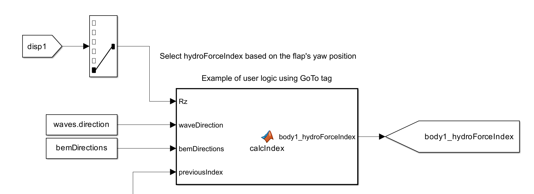
Note
Variable hydrodynamics is not compatible with the following features:
State-space radiation calculations
FIR Filter radiation calculations
Generalized body modes
Non-hydrodynamic and drag bodies
Nonlinear hydrodynamics is not compatible when using a case with variable mass.
Impulse Response Function with Variable Hydrodynamics
The convolution integral formulation of the radiation force is typically defined by
The Convolution Integral Formulation section gives additional details on this representation of the radiation force.
Note that \(K_r\) is a function of time and can change as the state varies when using variable hydrodynamics.
For example, if the state switches from “A” to “B” between times \(t_1, t_2\), then \(K_r(t-t_1)=K_{r,A}(t-t_1)\) is from a different hydrodynamic dataset
than \(K_{r,B}(t-t_2)\). To account for this change in the impulse response function history, a surface of IRF coefficients is created and
stored in body.variableHydro.radiationIrfSurface.
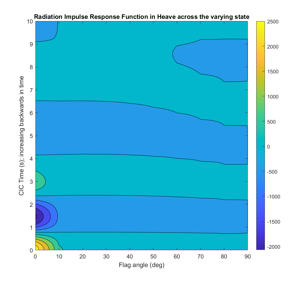
This 4D surface has dimensionsions of time, influenced degree of freedom, radiating degree of freedom, and varying state.
At each time step, convolutionIntegralSurface is called to evaluate the radiation force.
The time history of the varying state’s index is used to select the appropriate \(K_r\) coefficients given the time and state at that time.
The resulting 3D surface is then convolved with the velocity history and summed across the radiating degrees of freedom to give the radiation force at that time.
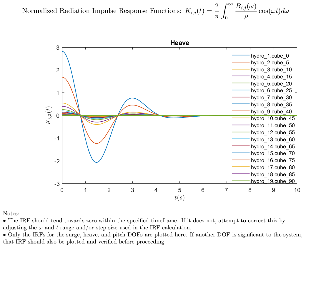
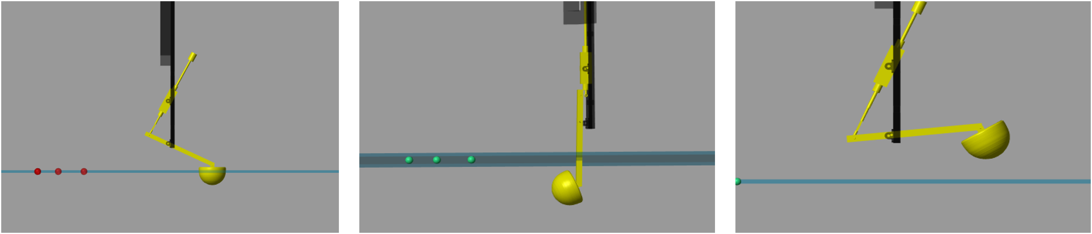
The two figures below show an example of how the radiation IRF varies across a state for the case of a single heaving cube whose base opens and closes. The flaps of the base split in half and are fully closed at 0 degrees and fully open at 90 degrees. The contour of IRF surface in heave illustrates how significantly the IRF coefficients can change with a varying state.
Application
See the Variable Hydrodynamics WEC-Sim_Application for a demonstration of setting up and using variable hydrodynamics.
Additional Considerations
Variable hydrodynamics is a complex feature that should be used with caution. Before using variable hydrodynamics, consider the advantages and disadvantages of other advanced features that can accomplish modeling goals effectively (passive yaw, large XY displacements, etc).
Thoroughly define the range of the state that is varying. Input BEM data to cover the entire range of the state. Sufficiently discretize the state to prevent numerical instabilities when switching occurs while reaching an acceptable computational expense. The Variable Hydro Passive Yaw application demonstrates how to process BEM datasets with BEMIO and interpolate between them to increase state resolution without requiring many BEM simulations. Due to the number of H5 files required, the hydroData directory may become very large.
All H5 files are loaded into the respective body variable, making the size
of these variables very large. Pre-processing remains very fast, so it is not
recommended to save body to an output file or the file size may increase drastically.
Body Initialization
The bodyClass is typically defined by inputting one or more paths to H5 files in the body constructor.
Alternatively, users may input a hydroData structure directly to the body constructor to bypass the
pre-processing steps that require writing the H5 file with BEMIO and then reloading it in the bodyClass.
This workflow may save users time in computationally expensive scenarios.
This alternate workflow is used by defining a body as: body(i) = bodyClass(hydroData).
Users should take care to ensure that the hydroData structure passed is identical in form to that
which initializeWecSim obtains by calling:
hydroData = readBEMIOH5('pathToH5File', body.number, body.meanDrift);
The function rebuildHydroStruct() may be used to convert the BEMIO hydro structure
into the bodyClass hydroData format.
Constraint and PTO Features
This section provides an overview of WEC-Sim’s constraint and PTO classes; for more information about the constraint and PTO classes’ code structure, refer to Constraint Class and PTO Class.
Modifying Constraints and PTOs
The default linear and rotational constraints and PTOs allow for heave and
pitch motions of the follower relative to the base. To obtain a linear or
rotational constraint in a different direction you must modify the constraint’s
or PTO’s coordinate orientation. The important thing to remember is that a
linear constraint or PTO will always allow motion along the joint’s Z-axis, and
a rotational constraint or PTO will allow rotation about the joint’s Y-axis. To
obtain translation along or rotation about a different direction relative to
the global frame, you must modify the orientation of the joint’s coordinate
frame. This is done by setting the constraint’s or PTO’s orientation.z
and orientation.y properties which specify the new direction of the Z-
and Y- joint coordinates. The Z- and Y- directions must be perpendicular to
each other.
As an example, if you want to constrain body 2 to surge motion relative to body
1 using a linear constraint, you would need the constraint’s Z-axis to point in
the direction of the global surge (X) direction. This would be done by setting
constraint(i).orientation.z=[1,0,0] and the Y-direction to any
perpendicular direction (can be left as the default y=[0 1 0]). In this
example, the Y-direction would only have an effect on the coordinate on which
the constraint forces are reported but not on the dynamics of the system.
Similarly if you want to obtain a yaw constraint you would use a rotational
constraint and align the constraint’s Y-axis with the global Z-axis. This would
be done by setting constraint(i).orientation.y=[0,0,1] and the
z-direction to a perpendicular direction (say [0,-1,0]).
Note
When using the Actuation Force/Torque PTO or Actuation Motion PTO blocks, the loads and displacements are specified in the local (not global) coordinate system. This is true for both the sensed (measured) and actuated (commanded) loads and displacements.
Additionally, by combining constraints and PTOs in series you can obtain different motion constraints. For example, a massless rigid rod between two bodies, hinged at each body, can be obtained by using a two rotational constraints in series, both rotating in pitch, but with different locations. A roll-pitch constraint can also be obtained with two rotational constraints in series; one rotating in pitch, and the other in roll, and both at the same location.
Incorporating Joint/Actuation Stroke Limits
Beginning in MATLAB 2019a, hard-stops can be specified directly for PTOs and
translational or rotational constraints by specifying joint-primitive dialog
options in the wecSimInputFile.m. Limits are modeled as an opposing spring
damper force applied when a certain extents of motion are exceeded. Note that
in this implementation, it is possible that the constraint/PTO will exceed
these limits if an inadequate spring and/or damping coefficient is specified,
acting instead as a soft motion constraint. More detail on this implementation
can be found in the Simscape documentation.
To specify joint or actuation stroke limits for a PTO, the following parameters
must be specified in wecSimInputFile.m:
pto(i).hardStops.upperLimitSpecify = 'on'
pto(i).hardStops.lowerLimitSpecify = 'on'
The specifics of the limit and the acting forces at the upper and lower limits are described in turn by:
pto(i).hardStops.upperLimitBound
pto(i).hardStops.upperLimitStiffness
pto(i).hardStops.upperLimitDamping
pto(i).hardStops.upperLimitTransitionRegionWidth
pto(i).hardStops.lowerLimitBound
pto(i).hardStops.lowerLimitStiffness
pto(i).hardStops.lowerLimitDamping
pto(i).hardStops.lowerLimitTransitionRegionWidth
where pto(i) is replaced with constraint(i) on all of the above if the limits are to be applied to a constraint.
In MATLAB versions prior to 2019a, specifying any of the above parameters will have no effect on the simulation, and may generate warnings. It is instead recommended that hard-stops are implemented in a similar fashion using an Actuation Force/Torque PTO block in which the actuation force is specified in a custom MATLAB Function block.
Setting PTO or Constraint Extension
The PTO and Constraint classes have an Extension value that
can be specified to define the initial displacement of
the PTO or constraint at the beginning of the simulation, allowing the user to set the
ideal position for maximum wave capture and energy generation. This documentation
will use the PTO as an example, but the proces is applicable to both translational,
rotational, or spherical PTOs and constraints.
Whereas the initial displacement feature only defines this updated position for the PTO,
the PTO Extension feature propagates the change in position to all bodies and joints
on the Follower side of the PTO block. This allows for an accurate reflection of the
initial locations of each component without having to calculate and individually
define each initial displacement or rotation. To set the extension of a PTO, the
following parameter must be specified in wecSimInputFile.m:
pto(i).extension.PositionTargetSpecify = '1'
to enable the joint’s target position value to be defined. The specifics of the extension are described in turn by:
pto(i).extension.PositionTargetValue
pto(i).extension.PositionTargetPriority
PositionTargetValue defines the extension magnitude and PositionTargetPriority
specifies Simulink’s priority in setting the initial target value in regards
to other constraints and PTOs. The priority is automatically set to “High” when
the extension is initialized but can be adjusted to “Low” if required by Simulink.
The figure below shows the PTO extension feature on the WECCCOMP model at 0.1 m.
The left image is at equilibrium (pto(i).extension.PositionTargetSpecify=0),
and the right image set as
pto(i).extension.PositionTargetSpecify=1 with the WEC body moving in
accordance with the set PTO Extension value.
WECCCOMP Model PTO Extension
While this method generally fits most WEC models, there are specific designs such as the RM3 that may have a larger DOF and are dependent on the particular block orientation in the simulink model in terms of which body blocks will move in response to a PTO initial extension. These specific cases require extra setup on the users end if looking to define a different body’s motion than the one automatically established. For the RM3 model, a set PTO Extension value results in movement in the float body. However, if the user would like the movement to be within the spar instead, extra steps are required. To view examples of how to set the PTO Extension for both the float as well as the spar view the RM3 PTO Extension examples on the WEC-Sim Applications repository .
For the spherical PTO which can rotate about three axes,
pto(i).extension.PositionTargetValue must be a 1x3 array that specifying
three consecutive rotations about the Base frame’s axes in the X-Y-Z convention.
Note
The PTO extension is not valid for PTO already actuated by user-defined motion (Translational PTO Actuation Motion, Rotational PTO Actuation Motion).
PTO-Sim
PTO-Sim is the WEC-Sim module responsible for accurately modeling a WEC’s conversion of mechanical power to electrical power. While the PTO blocks native to WEC-Sim are modeled as a simple linear spring-damper systems, PTO-Sim is capable of modeling many power conversion chains (PCC) such as mechanical and hydraulic drivetrains. PTO-Sim is made of native Simulink blocks coupled with WEC-Sim, using WEC-Sim’s user-defined PTO blocks, where the WEC-Sim response (relative displacement and velocity for linear motion and angular position and velocity for rotary motion) is the PTO-Sim input. Similarly, the PTO force or torque is the WEC-Sim input. For more information on how PTO-Sim works, refer to [So et al., 2015] and Series 3 - Non-hydrodynamic Bodies.
The files for the PTO-Sim tutorials described in this section can be found in the PTO-Sim examples on the WEC-Sim Applications repository . Four PTO examples are contained in the PTO-Sim application and can be used as a starting point for users to develop their own. They cover two WEC types and mechanical, hydraulic, and electrial PTO’s:
PTO-Sim Application
Description
RM3_cHydraulic_PTO
RM3 with compressible hydraulic PTO
RM3_DD_PTO
RM3 with direct drive linear generator
OSWEC_Hydraulic_PTO
OSWEC with hydraulic PTO (adjustable rod)
OSWEC_Hydraulic_Crank_PTO
OSWEC with hydraulic PTO (crank)
Tutorial: RM3 with PTO-Sim
This section describes how to use RM3 with PTO-Sim. Two tutorials will be given in this section: one for the RM3 with a hydraulic PTO and another for the RM3 with a direct drive PTO.
RM3 with Hydraulic PTO
The hydraulic PTO example used in this section consists of a piston, a rectifying valve, a high pressure accumulator, a hydraulic motor coupled to a rotary generator, and a low pressure accumulator.
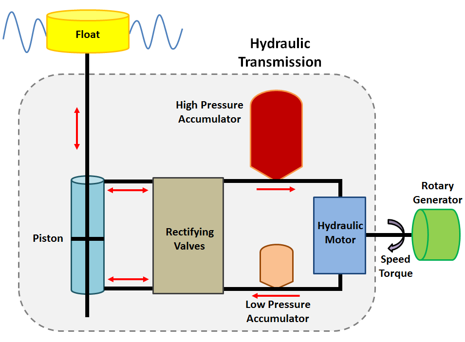
In this section, a step by step tutorial on how to set up and run the RM3
simulation with PTO-Sim is provided. All the files used in WEC-Sim will remain
the same, but some may need to be added to the working folder. The wecSimInputFile.m must
be modified to add the definition of the different PTO-Sim blocks. The files used to run RM3 with
PTO-Sim case are the following:
WEC-Sim input file:
wecSimInputFile.m(make sure to set the PTO linear damping to zero)Simulink model:
RM3.slxGeometry file for each body:
float.stlandplate.stlHydrodynamic data file(s):
rm3.h5Optional user defined post-processing file:
userDefinedFunction.m
Simulink Model
The Simulink model can be built as follows:
Step 1: Navigate to the RM3 example
$WECSIM/examples/RM3.Step 2: Open
RM3.slxfile and replace Translational PTO with Translational PTO Actuation Force.
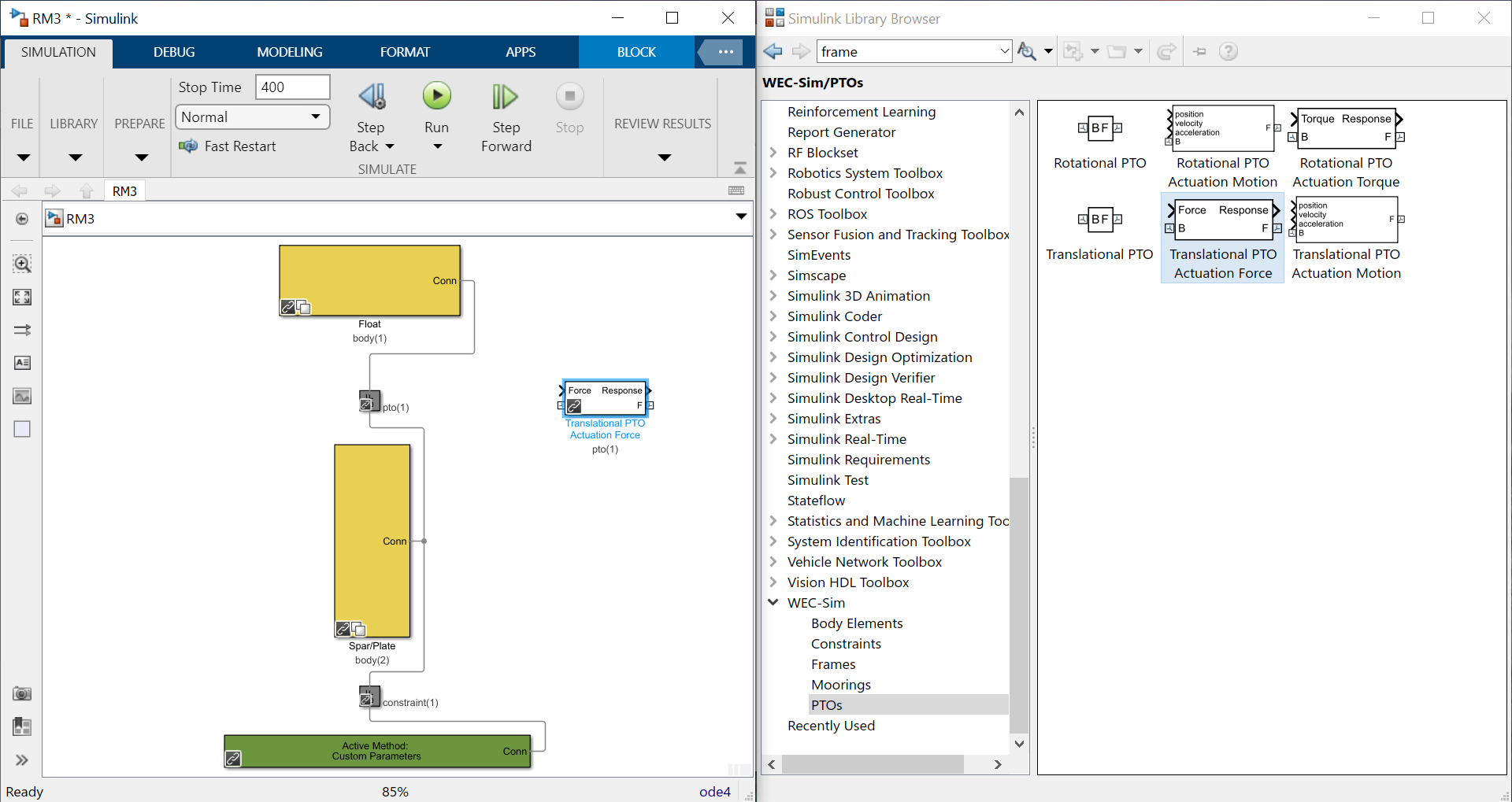
Step 3: Create a subsystem and rename it to PTO-Sim where the input is the response and output is force.
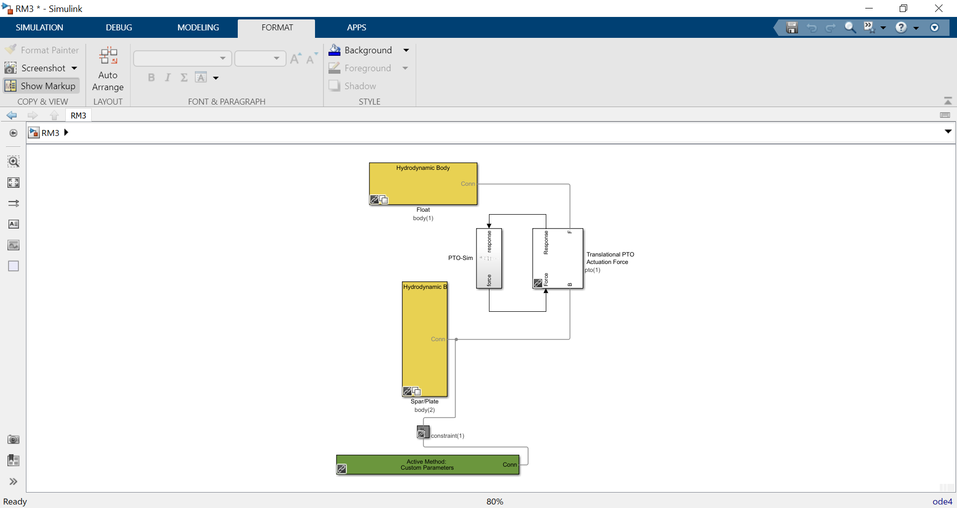
Step 4: Go to Simulink Library Browser to access the PTO-Sim Library.
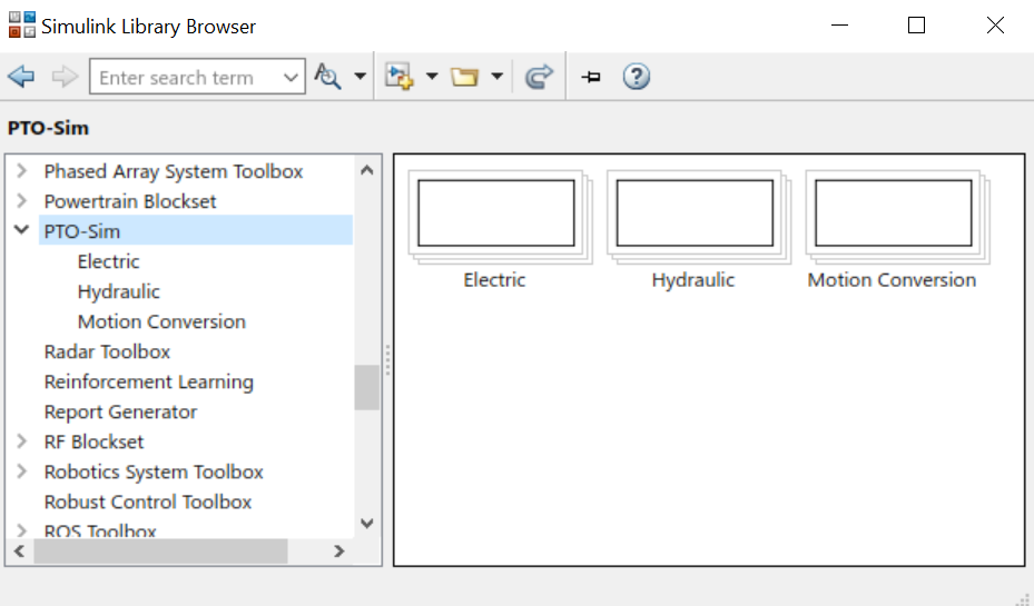
Step 5: By looking at the physical hydraulic PTO model as shown above, the user can simply drag and drop PTO-Sim library blocks. Hydraulic cylinder, rectifying valve, and accumulator blocks are located under the Hydraulic block. The electric generator equivalent circuit is located under the Electric library.
Step 6: Since multiple PTO-Sim blocks will be used, it is necessary to name each block to identify them when its variables are defined in the
wecSimInputFile.m. To change the name of each block, double click the block and add the nameptoSim(i)whereimust be different for each block used in the simulation. The name of each block will be used in thewecSimInputFile.mto define its variables.
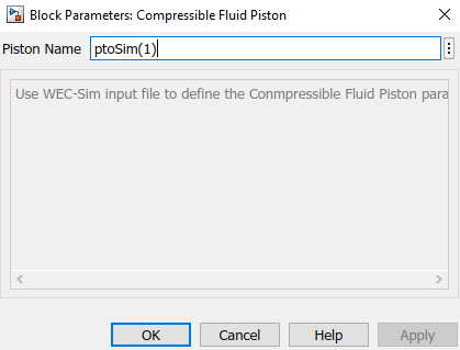
Step 7: Connect the inputs and outputs of the blocks according to the desired physical layout.
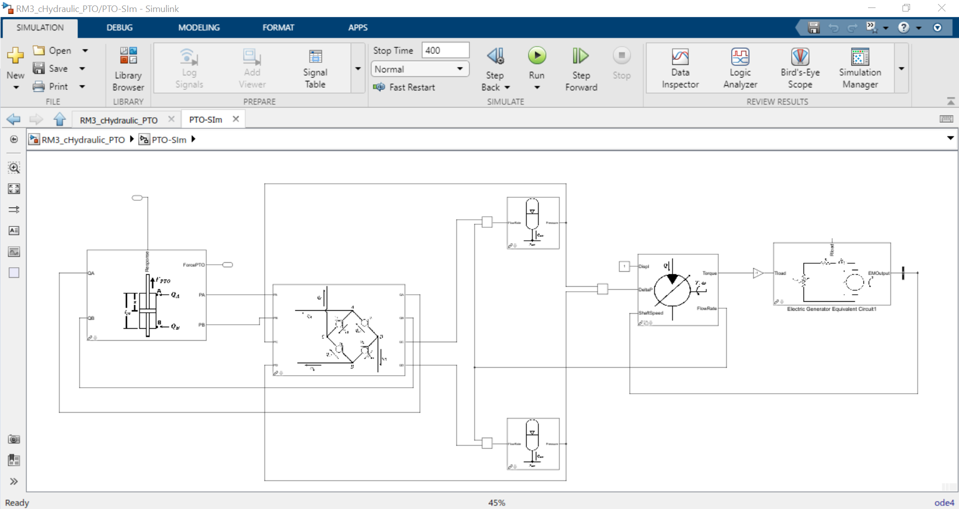
Step 8: Define the input for
Rloadin the Electric Generator block. The input could be a constant value or it could be used to control the load of the generator to achieve a desired physical behaviour. In this example, the value ofRloadis used to control the shaft speed of the generator by using a simple PI controller. The desired shaft speed in this case is 1000 rpm. The Electric Generator Equivalent Circuit block has two outputs: the electromagnetic torque and the shaft speed. It is necessary to use a bus selector to choose the desired output, which in this example is the shaft speed.
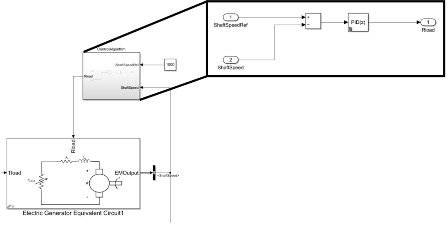
Input File
In this section, the WEC-Sim input file (wecSimInputFile.m) is defined and
categorized into sections such as hydraulic cylinder, rectifying check valve, high pressure
accumulator, low pressure accumulator, hydraulic motor, and generator.
%% Simulation Data
simu = simulationClass();
simu.simMechanicsFile = 'RM3_cHydraulic_PTO.slx'; %Location of Simulink Model File with PTO-Sim
simu.startTime = 0;
simu.rampTime = 100;
simu.endTime=400;
simu.dt = 0.01;
simu.explorer = 'off';                     % Turn SimMechanics Explorer (on/off)

%% Wave Information
%Irregular Waves using PM Spectrum
waves = waveClass('irregular');
waves.height = 2.5;
waves.period = 8;
waves.spectrumType = 'PM';
waves.phaseSeed=1;

%% Body Data
% Float
body(1) = bodyClass('../../../_Common_Input_Files/RM3/hydroData/rm3.h5');
body(1).geometryFile = '../../../_Common_Input_Files/RM3/geometry/float.stl';
body(1).mass = 'equilibrium';
body(1).inertia = [20907301 21306090.66 37085481.11];

% Spar/Plate
body(2) = bodyClass('../../../_Common_Input_Files/RM3/hydroData/rm3.h5');
body(2).geometryFile = '../../../_Common_Input_Files/RM3/geometry/plate.stl';
body(2).mass = 'equilibrium';
body(2).inertia = [94419614.57 94407091.24 28542224.82];

%% PTO and Constraint Parameters
% Floating (3DOF) Joint
constraint(1) = constraintClass('Constraint1');
constraint(1).location = [0 0 0];

% Translational PTO
pto(1) = ptoClass('PTO1');           	% Initialize PTO Class for PTO1
pto(1).stiffness = 0;                           % PTO Stiffness [N/m]
pto(1).damping = 0;                           % PTO Damping [N/(m/s)]
pto(1).location = [0 0 0];                   % PTO Location [m]

%% PTO new blocks

%Hydraulic Cylinder
ptoSim(1) = ptoSimClass('hydraulicCyl');
ptoSim(1).hydPistonCompressible.xi_piston = 35;
ptoSim(1).hydPistonCompressible.Ap_A = 0.0378;
ptoSim(1).hydPistonCompressible.Ap_B = 0.0378;
ptoSim(1).hydPistonCompressible.bulkModulus = 1.86e9;
ptoSim(1).hydPistonCompressible.pistonStroke = 70;
ptoSim(1).hydPistonCompressible.pAi = 2.1333e7;
ptoSim(1).hydPistonCompressible.pBi = 2.1333e7;

%Rectifying Check Valve
ptoSim(2) = ptoSimClass('rectCheckValve');
ptoSim(2).rectifyingCheckValve.Cd = 0.61;
ptoSim(2).rectifyingCheckValve.Amax = 0.002;
ptoSim(2).rectifyingCheckValve.Amin = 1e-8;
ptoSim(2).rectifyingCheckValve.pMax = 1.5e6;
ptoSim(2).rectifyingCheckValve.pMin = 0;
ptoSim(2).rectifyingCheckValve.rho = 850;
ptoSim(2).rectifyingCheckValve.k1 = 200;
ptoSim(2).rectifyingCheckValve.k2 = ...
    atanh((ptoSim(2).rectifyingCheckValve.Amin-(ptoSim(2).rectifyingCheckValve.Amax-ptoSim(2).rectifyingCheckValve.Amin)/2)*...
    2/(ptoSim(2).rectifyingCheckValve.Amax - ptoSim(2).rectifyingCheckValve.Amin))*...
    1/(ptoSim(2).rectifyingCheckValve.pMin-(ptoSim(2).rectifyingCheckValve.pMax + ptoSim(2).rectifyingCheckValve.pMin)/2);

%High Pressure Hydraulic Accumulator
ptoSim(3) = ptoSimClass('hydraulicAcc');
ptoSim(3).gasHydAccumulator.vI0 = 8.5;
ptoSim(3).gasHydAccumulator.pIprecharge = 2784.7*6894.75;

%Low Pressure Hydraulic Accumulator
ptoSim(4) = ptoSimClass('hydraulicAcc');
ptoSim(4).gasHydAccumulator.vI0 = 8.5;
ptoSim(4).gasHydAccumulator.pIprecharge = 1392.4*6894.75;

%Hydraulic Motor
ptoSim(5) = ptoSimClass('hydraulicMotor');
ptoSim(5).hydraulicMotor.effModel = 2;
ptoSim(5).hydraulicMotor.displacement = 120;
ptoSim(5).hydraulicMotor.effTableShaftSpeed = linspace(0,2500,20);
ptoSim(5).hydraulicMotor.effTableDeltaP = linspace(0,200*1e5,20);
ptoSim(5).hydraulicMotor.effTableVolEff = ones(20,20)*0.9;
ptoSim(5).hydraulicMotor.effTableMechEff = ones(20,20)*0.85;

%Electric generator
ptoSim(6) = ptoSimClass('electricGen');
ptoSim(6).electricGeneratorEC.Ra = 0.8;
ptoSim(6).electricGeneratorEC.La = 0.8;
ptoSim(6).electricGeneratorEC.Ke = 0.8;
ptoSim(6).electricGeneratorEC.Jem = 0.8;
ptoSim(6).electricGeneratorEC.bShaft = 0.8;
Simulation and Post-processing
Simulation and post-processing are similar process as described in Two-Body Point Absorber (RM3).
There are some specific variable definitions that must be considered when using the output
signals of the PTO-Sim blocks. For example, the hydraulic accumulator has two output signals: flow rate
and pressure, and the time vector. In the RM3 example with hydraulic PTO, the high pressure hydraulic
accumulator was defined as ptoSim(3) in the WEC-Sim input file; then, to use the output
flow rate and pressure of this block, the next line of code must be used:
FlowRateAccumulator = output.ptoSim(3).FlowRate
PressureAccumulator = output.ptoSim(3).Pressure
In general, the output signal of any PTO-Sim block can be used with this line of code: output.ptoSim(i).VariableName
RM3 with Direct Drive PTO
A mechanical PTO is used in this example and is modeled as a direct drive linear generator. The main components of this example consist of magnets and a coil where the magnet assembly is attached to the heaving float and the coil is located inside the spar. As the float moves up and down, the magnet assembly creates a change in the magnetic field surrounding the spar that contains the coil: therefore, current is induced in the coil and electricity is generated.
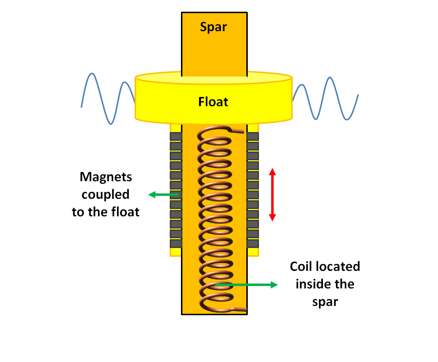
Simulink Model
Steps 1 through 4 are the same as in RM3 with Hydraulic PTO.
Step 5: Look for the block “Direct Drive Linear Generator” and drag the block into the PTO-Sim subsystem
Step 6: Connect the input “respose” to the input of the PTO-Sim block and the output “Force” to the output of the subsystem.
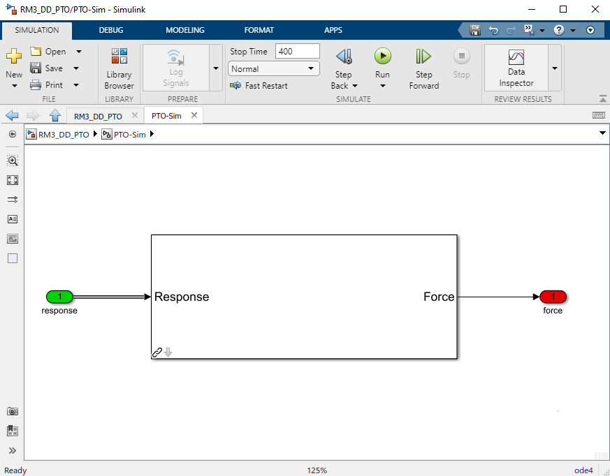
Input File, Simulation, and Post-processing
The same as RM3 with Hydraulic PTO.
Tutorial: OSWEC with PTO-Sim
This section describes how to use the OSWEC model with PTO-Sim. The same process as described in RM3 with Hydraulic PTO; however, since the OSWEC is a rotary device, it takes torque as an input and a rotary to linear motion conversion block is needed. The tutorials can be found on the WEC-Sim Applications repository (both for a crank and for a rod).
OSWEC with Hydraulic PTO
A hydraulic PTO or mechanical PTO can be used with OSWEC but for simplicity a hydraulic PTO will be used as an example. An schematic representation of the OSWEC device is shown in the figure below:
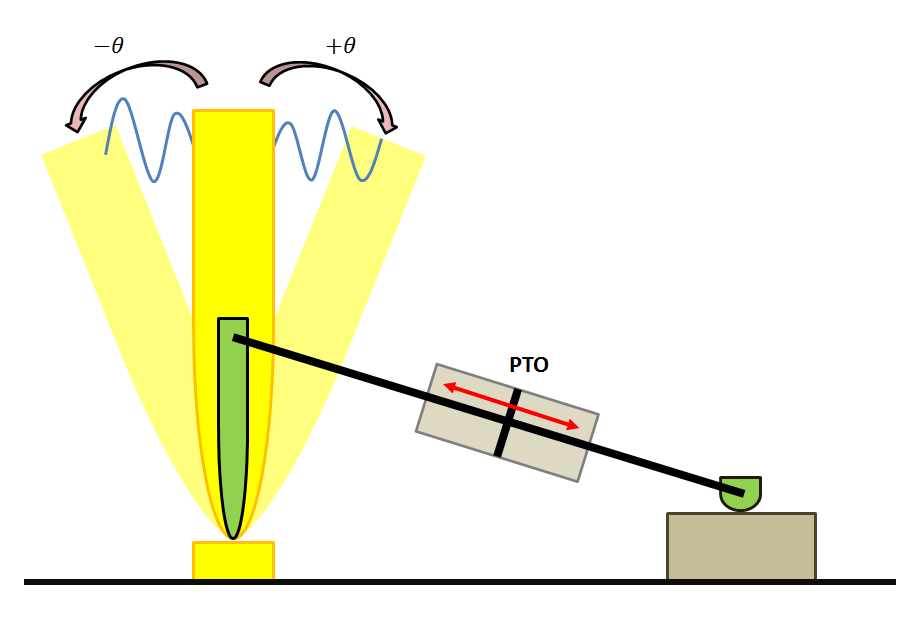
Two blocks were developed in the PTO-Sim library to model a system like the OSWEC.
The blocks can be found under the Motion Convertion library.
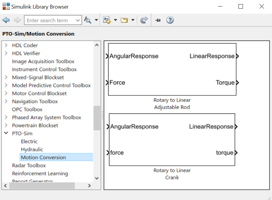
The block “Rotary to Linear Adjustable Rod” is used to model a rod with a variable length. For the OSWEC case, this block can be use when the cylinder rod of the hydraulic PTO is connected to the adjustable rod, like in the schematic presented in the figure below:
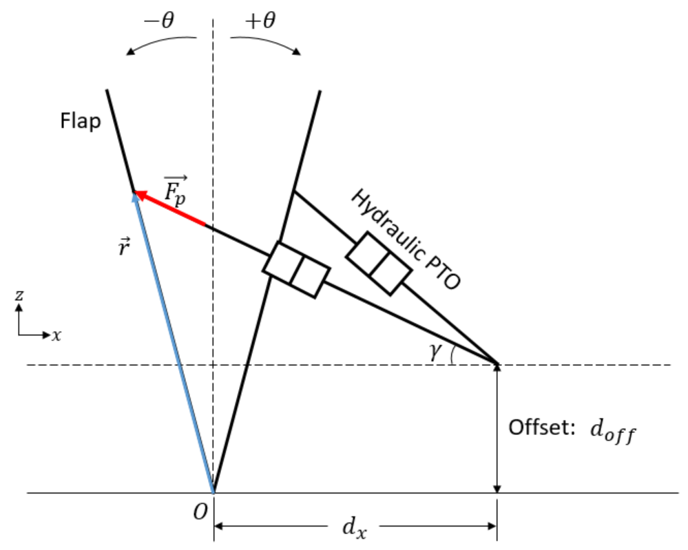
On the other hand, the block “Rotary to Linear Crank” is used to model a slider-crank mechanism that is used to convert the rotational motion of the OSWEC device into linear motion for the hydraulic cylinder in the PTO. In this case, the cylinder rod of the hydraulic PTO is connected to the slider part of the mechanism, as shown in the figure below:
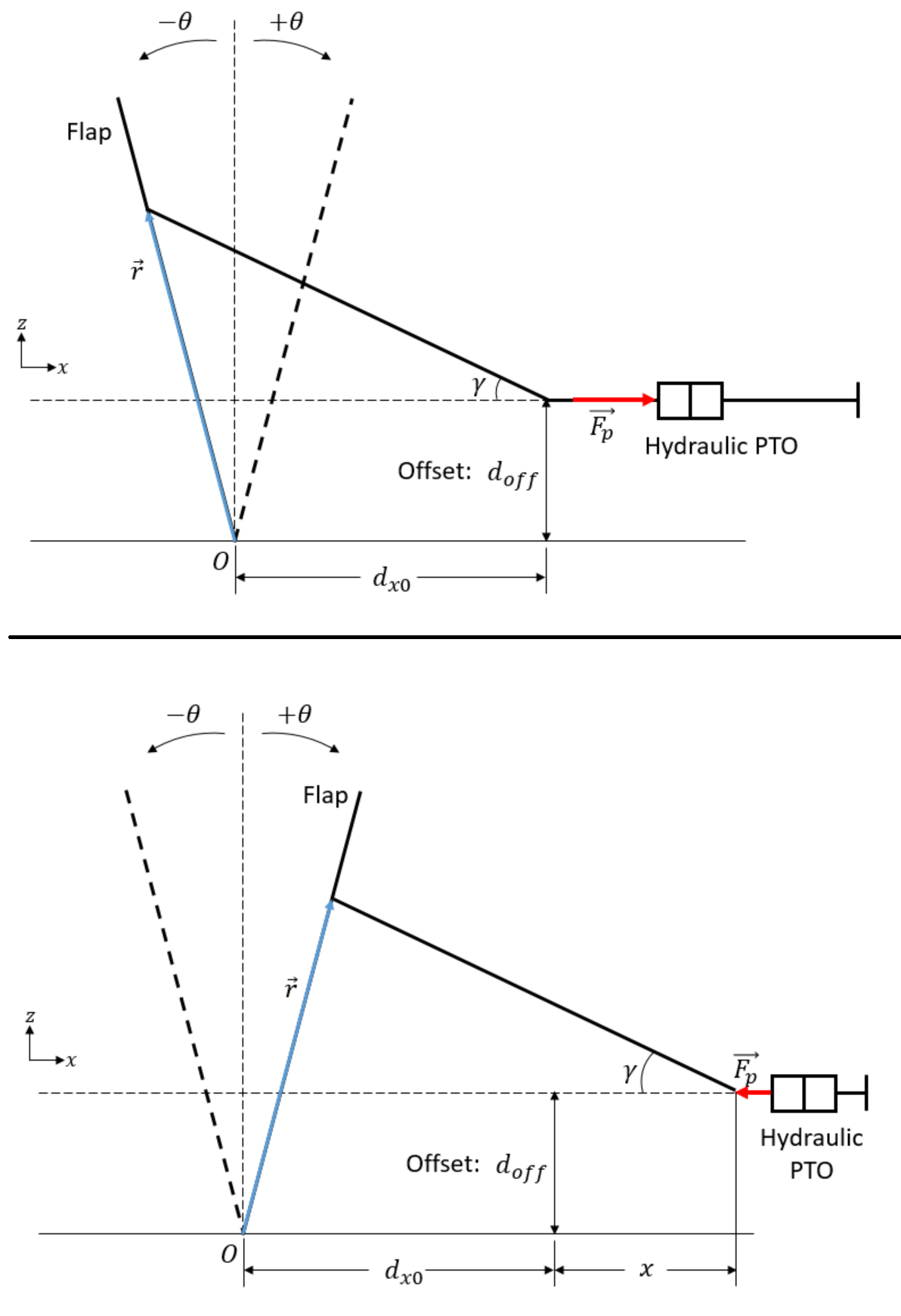
Modeling of OSWEC with Hydraulic PTO
The files needed for the OSWEC case are the same as the ones described in RM3 with Hydraulic PTO.
Simulink Model
The Simulink model can be built as following:
Step 1: Copy the OSWEC example folder to get started
$WECSIM\examples\OSWEC.Step 2: Open
OSWEC.slxfile and replace Rotational PTO with Rotational PTO Actuation Torque.
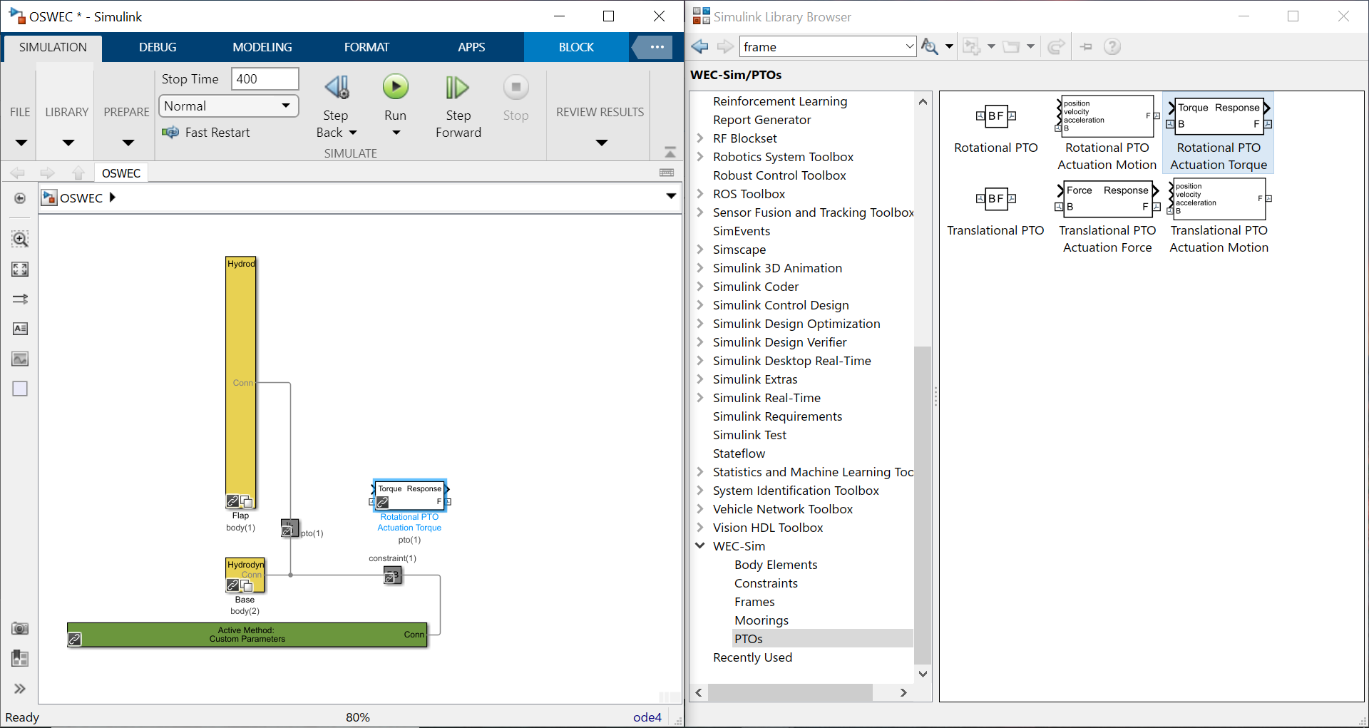
Step 3: Create a subsystem and rename it to PTO-Sim where input is response and output is torque.
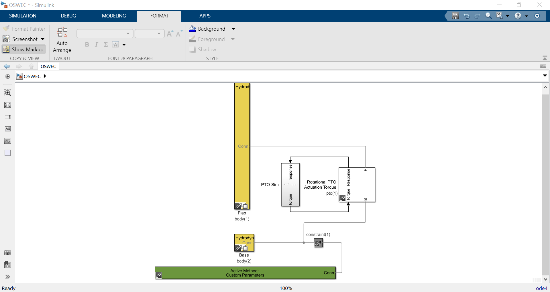
Step 4: Go to Simulink Library Browser to access the PTO-Sim Library.
Step 5: By looking at the physical hydraulic PTO model as shown above, the user can simply drag and drop PTO-Sim library blocks. Hydraulic cylinder, rectifying valve, and accumulator blocks are located under the Hydraulic block. The electric generator equivalent circuit is located under the Electric library. The “Rotary to Linear Adjustable Rod” is under the Motion Conversion library.
Step 6: Since multiple PTO-Sim blocks will be used, it is necessary to name each block to identify them when its variables are defined in the
wecSimInputFile.m. To change the name of each block, double click the block and add the nameptoSim(i)whereimust be different for each block used in the simulation. The name of each block will be used in thewecSimInputFile.mto define its variables. For this example, the motion conversion block will be calledptoSim(1)
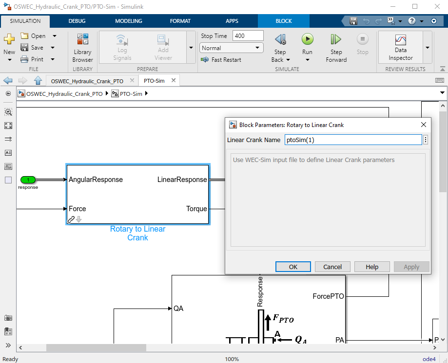
Step 7: Connect the inputs and outputs of the blocks according to the desired physical layout.
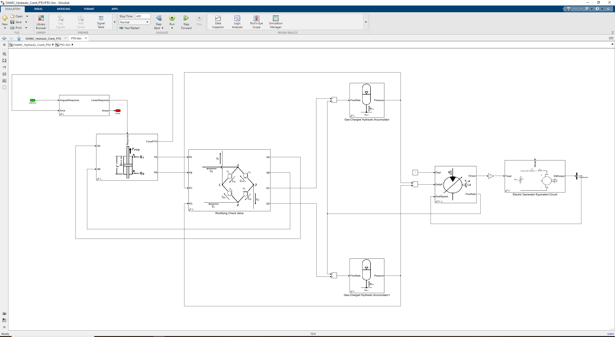
Step 8: Define the input for
Rloadin the Electric Generator block. The input could be a constant value or it could be used to control the load of the generator to achieve a desired physical behaviour. In this example, the value ofRloadis used to control the shaft speed of the generator by using a simple PI controller. The desired shaft speed in this case is 3000 rpm. The Electric Generator Equivalent Circuit block has two outputs: the electromagnetic torque and the shaft speed. It is necessary to use a bus selector to choose the desired output, which in this example is the shaft speed.
Input File, Simulation, and Post-processing
The input file for this case is similar to the input file described in RM3 with Hydraulic PTO. The naming and numbering of the PTO blocks change in this case, but the way the variables are defined is the same.
Controller Features
The power generation performance of a WEC is highly dependent on the control algorithm used in the system. There are different control strategies that have been studied for marine energy applications. These control algorithms can be applied directly to the PTO components to achieve a desired output, or they can be high-level controllers which are focused on the total PTO force applied to the WEC. The examples presented in this section are based on high- level controller applications. WEC-Sim’s controller features support the modeling of both simple passive and reactive controllers as well as more complex methods such as model predictive control.
The files for the controller tutorials described in this section can be found in the Controls examples on the WEC-Sim Applications repository . The controller examples are not comprehensive, but provide a reference for user to implement their own controls.
Controller Application
Description
Passive (P)
Sphere with proportional control
Reactive (PI)
Sphere with proportional-integral control
Latching
Sphere with latching control
Declutching
Sphere with declutching control
Model Predictive Control
Sphere with model predictive control
Reactive with PTO
Sphere with reactive control and DD PTO
Examples: Sphere Float with Various Controllers
First, it is important to understand the concept of complex conjugate control. Complex conjugate control, as applied to wave energy conversion, can be used to understand optimal control. For a complex conjugate controller, the impedance of the controller is designed to match the admittance of the device (equal to the complex conjugate of device impedance). Hence, it is also known as impedance matching and is a common practice within electrical engineering. Complex conjugate control is not a completely realizable control method due to its acausality, which means it requires exact knowledge of future wave conditions. Still, a causal transfer function can be used to approximate complex conjugate control across a limited frequency range [C1]. Thus, complex conjugate control presents a reference for the implementation of optimal causal controls. The WEC impedance can be modeled by the following equation [C2] and can be used to formulate the optimal control implementation:
By characterizing the impedance of the WEC, a greater understanding of the dynamics can be reached. The figure below is a bode plot of the impedance of the RM3 float body. The resonant frequency is defined by the point at which the phase of impedance is zero. By also plotting the frequency of the incoming wave, it is simple to see the difference between the resonant frequency of the device and the wave frequency. Complex conjugate control (and some other control methods) seeks to adjust the resonant frequency of the system to match the wave frequency. Matching the reonance frequency to the wave frequency leads to system resonance, which allows for theoretically optimal mechanical power.
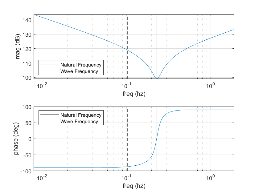
It is important to note here that although impedance matching can lead to maximum mechanical power, it does not always lead to maximum electrical power. Resonance due to impedance matching often creates high peaks of torque and power, which are usually far from the most efficient operating points of PTO systems used to extract power and require those systems to be more robust and expensive. Thus, the added factor of PTO dynamics and efficiency may lead to complex conjugate control being suboptimal. Furthermore, any constraints or other nonlinear dynamics may make complex conjugate control unachievable or suboptimal. Theoretical optimal control using complex conjugates presented here should be taken as a way to understand WEC controls rather than a method to achieve optimal electrical power for a realistic system.
Passive Control (Proportional)
Passive control is the simplest of WEC controllers and acts as a damping force. Hence, the damping value (also referred to as a proportional gain) is multiplied by the WEC velocity to determine the power take-off force:
Although unable to reach optimal power for a regular wave due to its passive nature, a passive controller can still be tuned to reach its maximum power. According to complex conjugate control, a passive controller can be optimized for regular wave conditions using the following formula [C3]:
The optimal proportional gain has been calculated for the float using the optimalGainCalc.m file and implemented in WEC-Sim to achieve optimal power. The mcrBuildGains.m file sets up a sweep of the proportional gains which can be used to show that the results confirm the theoretical optimal gain in the figure below (negative power corresponding to power extracted from the system). This MCR run can be recreated by running the mcrBuildGains.m file then typing wecSimMCR in the command window.
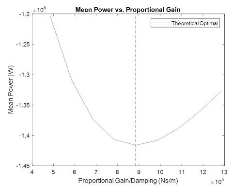
This example only shows the optimal proportional gain in regular wave conditions. For irregular wave spectrums and nonlinear responses (such as with constraints), an optimization algorithm can be used to determine optimal control gains.
Reactive Control (Proportional-Integral)
Reactive control is also a very simple form of WEC control and combines the damping force of a passive controller with a spring stiffness force. The standard PTO block can also be used to implement PI control using the damping and stiffness values but doesn’t allow for negative inputs which is often necessary for optimal stiffness. This controller is also known as a proportional integral controller with the proportional gain corresponding to the damping value and the integral gain corresponding to a spring stiffness value:
The addition of the reactive component means the controller can achieve optimal complex conjugate control by cancelling out the imaginary portion of the device impedance. Thus, the proportional and integral control gains can be defined by the following formulas [C4]:
The optimal proportional and integral gains have been calculated using the optimalGainCalc.m file and implemented in WEC-Sim to achieve optimal power. The mcrBuildGains.m file again sets up a sweep of the gains which can be used to show that the results confirm the theoretical optimal gains in the figure below. This MCR run can be recreated by running the mcrBuildGains.m file then typing wecSimMCR in the command window.
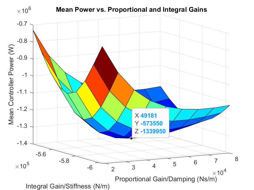
This example only shows the optimal gains in regular wave conditions. For irregular wave spectrums and nonlinear responses (such as with constraints), an optimization algorithm can be used to determine optimal control gains.
Latching Control
Latching control combines a traditional passive controller with a latching mechanism which applies a large braking force during a portion of the oscillation. By locking the device for part of the oscillation, latching control attempts to adjust the phase of the motion to match the phase of incoming waves. Latching control can slow the device motion to match wave motion and is therefore most often used when the wave period is longer than the resonant period. Latching control is still considered passive as no energy input is required (assuming velocity is zero while latched).
The braking/latching force is implemented as a very large damping force (\(G\)), which can be adjusted based on the device’s properties [C5]:
Because latching achieves phase matching between the waves and device, the optimal damping can be assumed the same as for reactive control. Lastly, the main control variable, latching time, needs to be determined. For regular waves, it is desired for the device to move for a time equal to its resonant frequency, meaning the optimal latching time is likely close to half the difference between the wave period and the resonant period [C5] (accounting for 2 latching periods per wave period).
The optimal latching time has been calculated using the optimalGainCalc.m file and implemented in WEC-Sim. The mcrBuildTimes.m file sets up a sweep of the latching times, the results for which are shown in the figure below. This MCR run can be recreated by running the mcrBuildGains.m file then typing wecSimMCR in the command window. Based on the results, the optimal latching time is slightly lower than expected which may be due to imperfect latching or complex dynamics which aren’t taken into account in the theoretical optimal calculation. Regardless, latching results in much larger power when compared to traditional passive control.
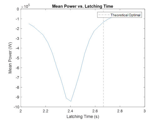
Further, the figure below shows the excitation force and velocity, which are close to in phase when a latching time of 2.4 seconds is implemented.
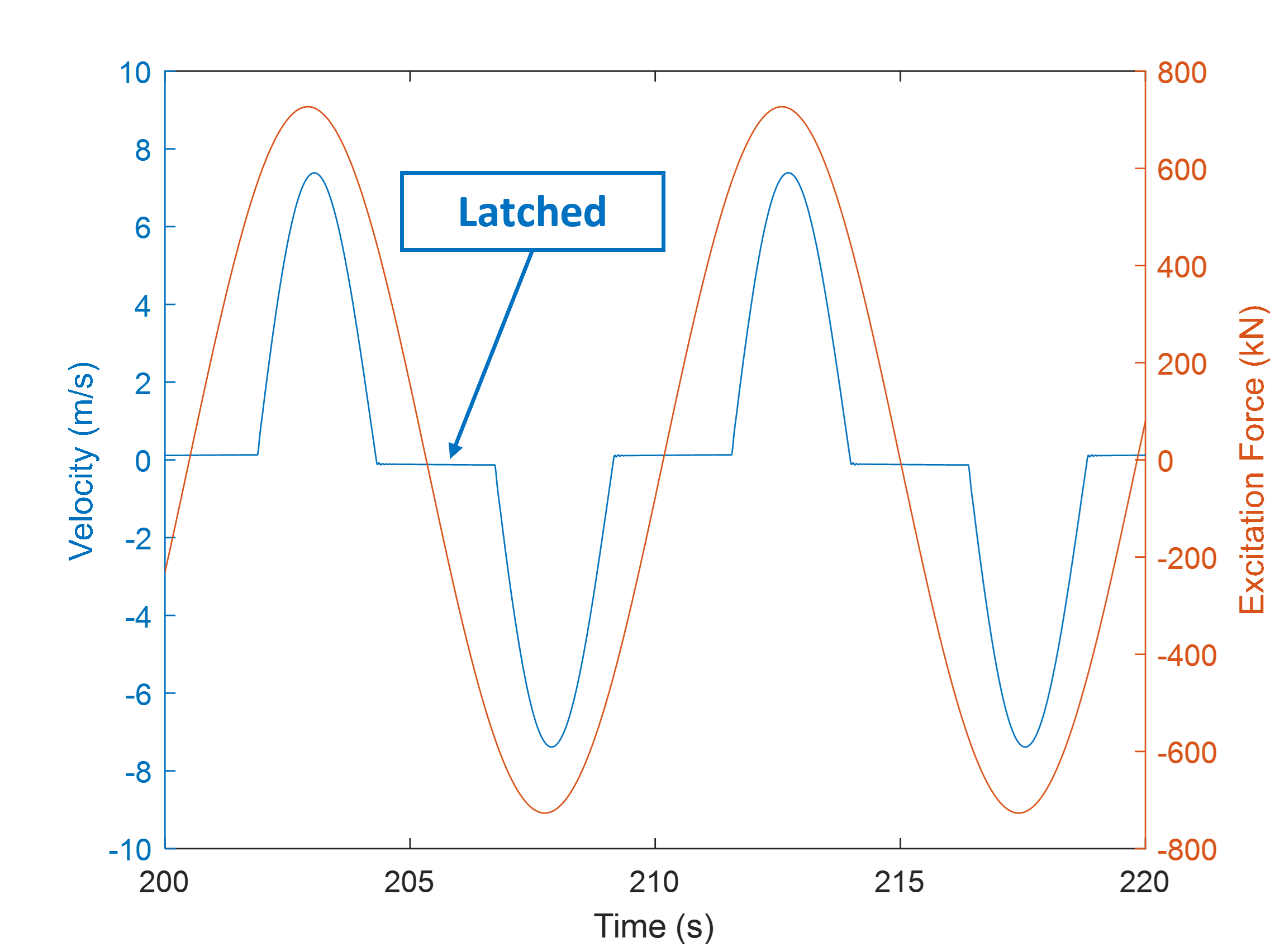
Although not shown with this example, latching can also be implemented in irregular waves but often requires different methods including excitation prediction.
Declutching Control
Declutching control is essentially the opposite of latching. Instead of locking the device, it is allowed to move freely (no PTO force) for a portion of the oscillation. Often, declutching is used when the wave period is smaller than the resonant period, allowing the device motion to “catch up” to the wave motion. Declutching is also considered a passive control method.
The optimal declutching time and damping values are slightly harder to estimate than for latching. The device’s motion still depends on its impedance during the declutching period, meaning the device does not really move “freely” during this time. Hence, in opposition to optimal latching the declutching time was assumed to be near half the difference between the resonant period and the wave period, but is further examined through tests.
This optimal declutching time has been calculated using the optimalGainCalc.m file and implemented in WEC-Sim. Because energy is not harvested during the declutching period, it is likely that a larger damping is required. Thus, the optimal passive damping value was used for the following simulations, although a more optimal damping value likely exists for delclutching.
Since declutching is most desired when the wave period is smaller than the resonant period, a wave period of 3.5 seconds was tested with a height of 1 m. For comparison to traditional passive control, the optimal passive damping value was tested for these conditions, leading to a power of 5.75 kW. The mcrBuildTimes.m file sets up a sweep of the declutching times, the results for which are shown in the figure below. It is clear that delcuthing control can offer an improvement over traditional passive control.
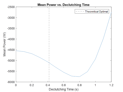
Further, the figure below shows the excitation force and velocity with a declutch time of 0.8 seconds. The excitation and response are not quite in phase, but the device can be seen “catching up” to the wave motion during the declutching time.
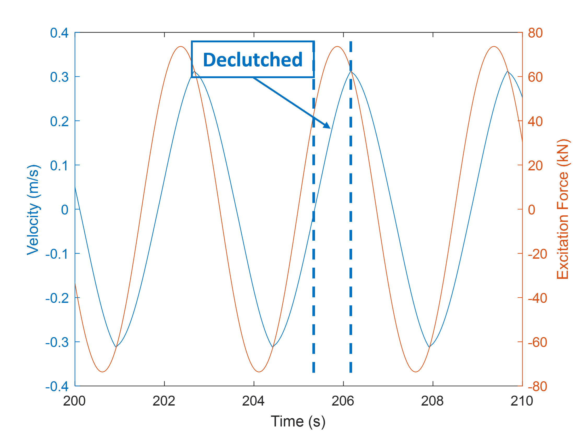
Although not shown with this example, declutching can also be implemented in irregular waves but often requires different methods including excitation prediction.
Model Predictive Control (MPC)
Model predictive control is a WEC control method which uses a plant model to predict and optimize the dynamics. MPC is a complex controller that can be applied in both regular and irregular waves while also taking into account time-domain constraints such as position, velocity, and PTO force. For the model predictive controller implemented here, the plant model is a frequency dependent state-space model [C6]. The state space model is then converted to a quadratic programming problem to be solved by quadprog(), MATLAB’s quadratic programming function. Solving this system leads to a set of PTO forces to optimize the future dynamics for maximum harvested power, the first of which is applied at the current timestep. The relevant files for the MPC example in the Controls folder of WEC-Sim Applications are detailed in the table below (excluding wecSimInputFile.m and userDefinedFunctions.m which are not unique to MPC). Note: This controller is similar to the NMPC example within the WECCCOMP Application, but this example includes a method for calculating frequency dependence and setting up the state space matrices based on boundary element method data, allows for position, velocity, and force constraints, and is applied to a single body heaving system.
File
Description
coeff.mat
Coefficients for frequency dependence
fexcPrediction.m
Predicts future excitation forces
sphereMPC.slx
Simulink model including model predictive controller
mpcFcn.m
Creates and solves quadratic programming problem
plotFreqDep.m
Solves for and plots frequency dependence coeffs
The Simulink diagram is shown in the figure below. The figure shows an overview of the controller, which primarily consists of the plant model and the optimizer. The plant model uses the excitation force, applied PTO force, and current states to calculate the states at the next timestep. Then, the optimizer predicts the future excitation, which is input into the mpcFcn.m file along with the states to solve for the optimal change in PTO force (integrated to solve for instantaneous PTO force).
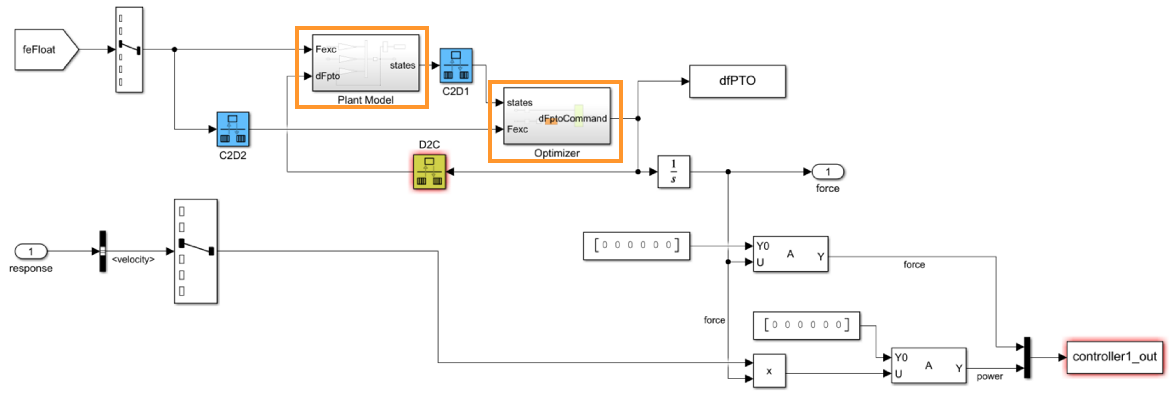
The results of the model predictive controller simulation in irregular waves are shown below with the dashed lines indicating the applied constraints. MPC successfully restricts the system to within the constraints (except for a few, isolated timesteps where the solver couldn’t converge) while also optimizing for maximum average mechanical power (300 kW). The constraints can be changed to account for specific WEC and PTO physical limitations, but will limit the average power. There are also other parameters which can be defined or changed by the user in the wecSimInputFile.m such as the MPC timestep, prediction horizon, r-scale, etc. to customize and tune the controller as desired.
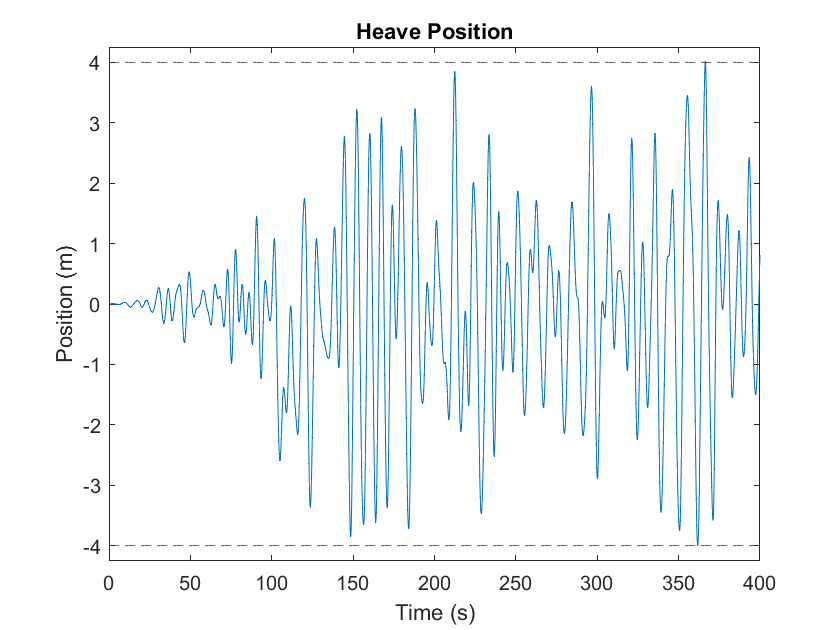
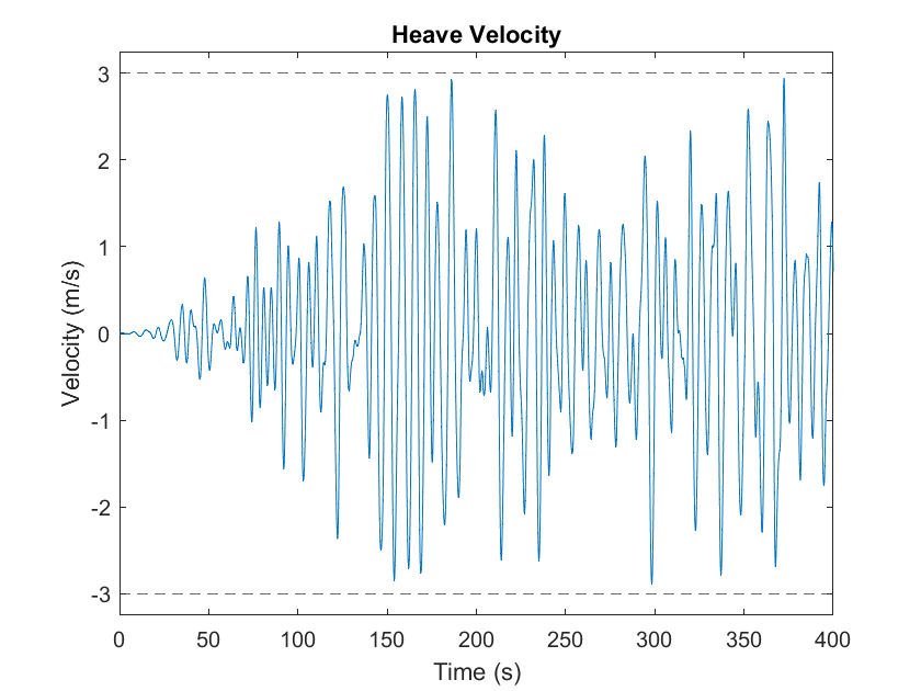
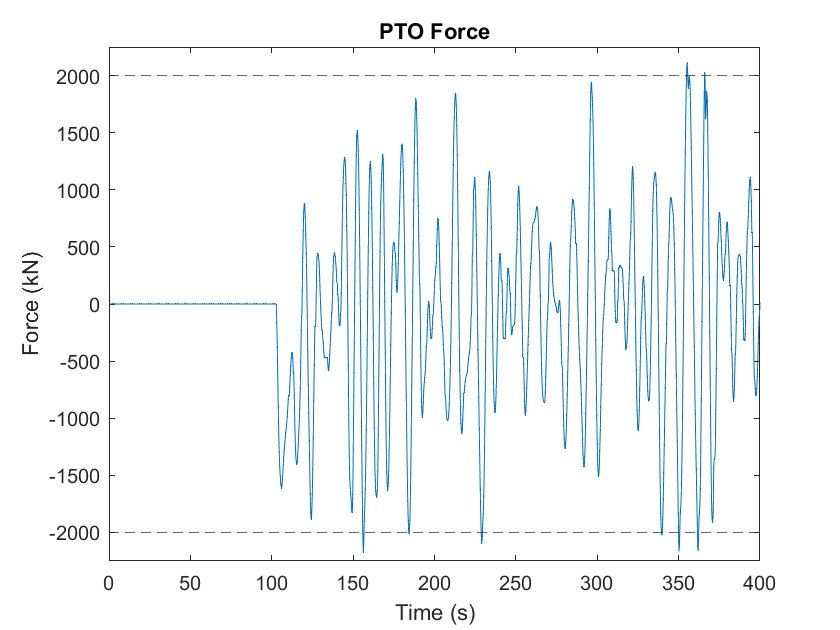
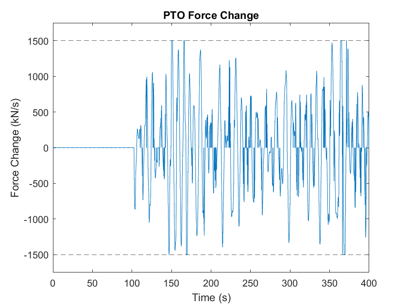
The model predictive controller is particularly beneficial because of its ability to predict future waves and maximize power accordingly as well as the ability to handle constraints. A comparison to a reactive controller is shown in the table below. The reactive controller can be tuned to stay within constraint bounds only when future wave conditions are known and, in doing so, would sacrifice significant power. On the other hand, without knowledge of future wave, the results from the untuned reactive controller are shown below using optimal theoretical gains from the complex conjugate method at the peak wave period. With no ability to recognize constraints, the reactive controller leads to much larger amplitude and velocity and exhibits large peaks in PTO force and power, both of which would likely lead to very expensive components and inefficient operation. It is clear that the model predictive controller significantly outperforms the reactive controller in terms of mechanical power harvested, constraint inclusions, and peak conditions. Because of the increased complexity of model predictive control, limitations include longer computation time and complex setup.
Parameter
Constraint
MPC
Reactive
Max Heave Position (m)
4
4.02
8.06
Max Heave Velocity (m/s)
3
2.95
5.63
Max PTO Force (kN)
2,000
2,180
4,630
Max PTO Force Change (kN/s)
1,500
1,500
3,230
Peak Mechanical Power (kW)
N/A
4,870
13,700
Avg Mechanical Power (kW)
N/A
300
241
Reactive Control with Direct Drive Power Take-Off
The previous controllers only considered the mechanical power output. Although maximization of mechanical power allows for the maximum energy transfer from waves to body, it often does not lead to maximum electrical power. The previous controller examples demonstrate the controller types and energy transfer from waves to body, but the important consideration of electrical power requires a PTO model. This example applies a reactive controller to the sphere body with a simplified direct drive PTO model to maximize electrical power. Within the Simulink subsystem for determining the PTO force, the controller prescribes the ideal or desired force which is fed into the direct drive PTO. The current in the generator is then used to control the applied force.
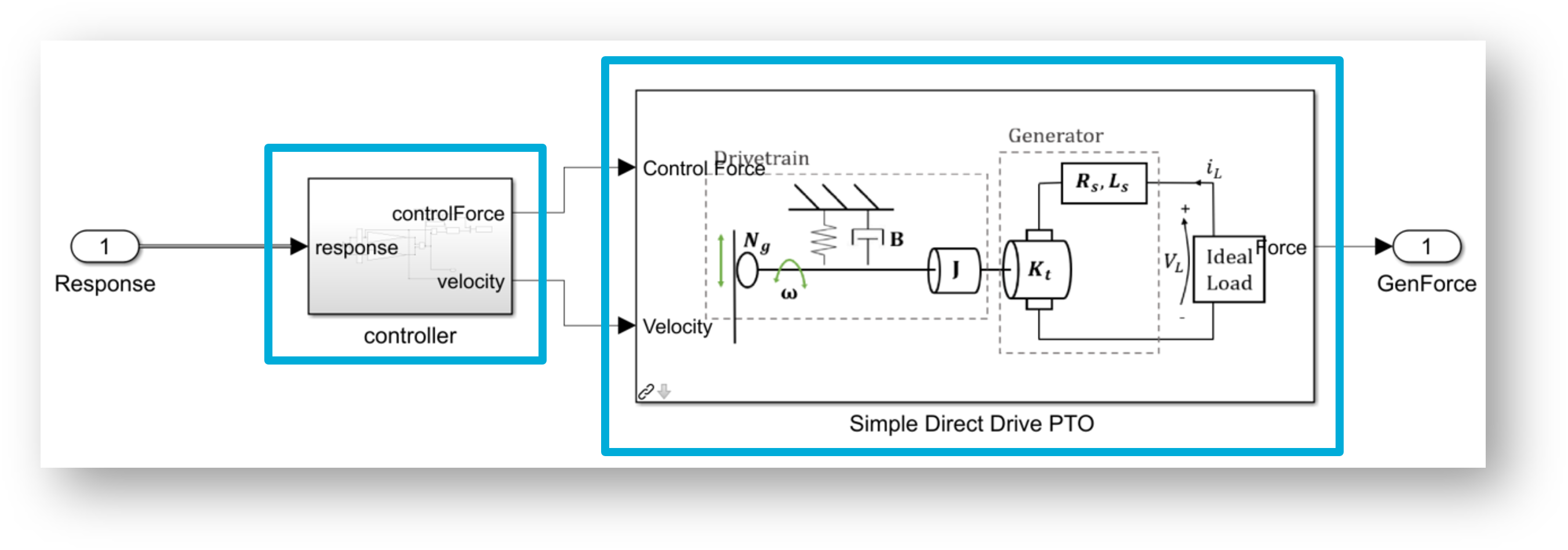
The PTO parameters used for this example are defined in the wecSimInputFile.m and correspond to
the Allied Motion Megaflux Frameless Brushless Torque Motors–MF0310 [C7]. The
results in terms of capture width (ratio of absorbed power (W) to wave power (W/m)) and resultant power for the
applied gains from Section Reactive Control (Proportional-Integral) are shown in the figures
below for a regular wave with a period of 9.6664 s and a height of 2.5 m. The “Controller (Ideal)”
power is the ideal power absorbed according to the applied controller gains.
The “Mechanical (Drivetrain)” power is the actual mechanical power absorbed by
the PTO system including the inertial, damping, and shaft torque power. Lastly, the
“Electrical (Generator)” power is the electrical power absorbed by the
generator including the product of induced current and voltage (based on shaft torque and velocity,
respectively) and the resultant generator losses (product of current squared and winding resistance).
Mechanical power maximization requires significant net input electrical power
(signified by red bar) which leads to an extremely negative capture width. Thus,
instead of harvesting electrical power, power would need to be taken from the grid or energy
storage component to achieve mechanical power maximization.
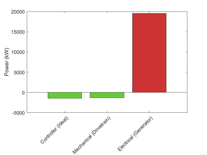
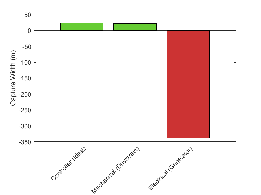
On the other hand, by testing different controller gains in the same wave conditions (regular wave: period = 9.6664 s, height = 2.5 m), the gains which optimize for maximum electrical power can be found as shown below. Increasing the proportional gain and decreasing the integral gain magnitude leads to a maximum power of about 84 kW and capture width of about 1.5 m. The resultant motion is almost ten times smaller than for the mechanical power maximization which leads to a lower current and much lower generator power losses (product of current squared and winding resistance).
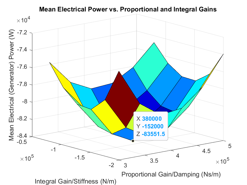
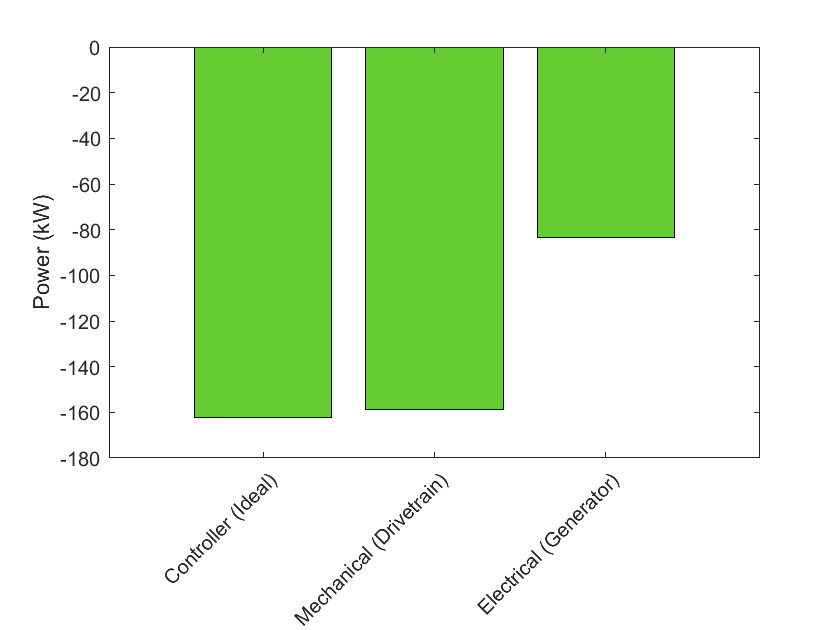
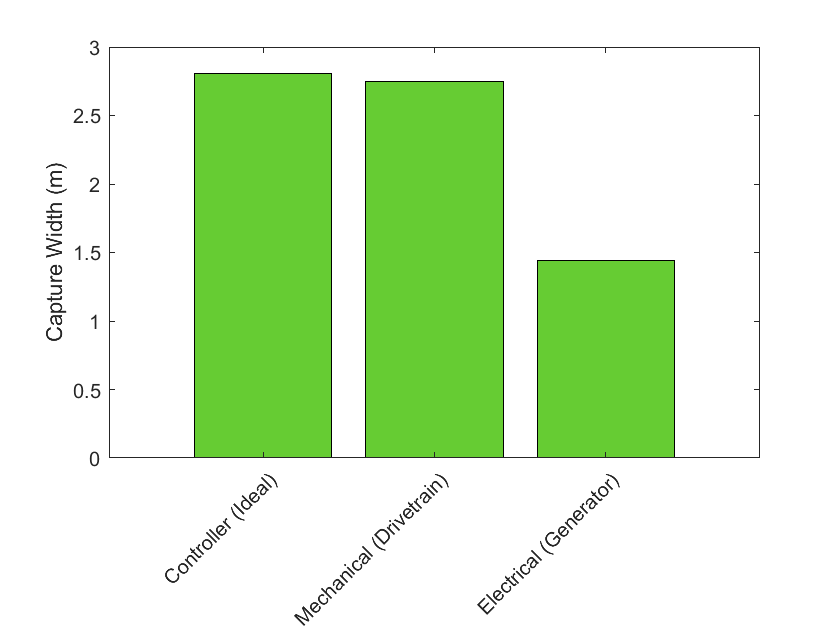
Cable Features
Cables or tethers between two bodies apply a force only in tension (when taut or stretched), but not in compression,
can be modeled using the cableClass implementation. A cable block must be added to the
model between the two PTOs or constraints that are to be connected by a cable. Users must initialize the cable
class in the wecSimInputFile.m along with the base and follower connections in that order, by including the following lines:
cable(i) = cableClass('cableName','baseConnection','followerConnection');
where baseConnection is a PTO or constraint block that defines the cable connection on the base side, and followerConnection
is a PTO or constraint block that defineds the connection on the follower side.
It is necessary to define, at a minimum:
cable(i).stiffness = <cableStiffness>;
cable(i).damping = <cableDamping>;
where cable(i).stiffness is the cable stiffness (N/m), and cable(i).damping is the cable damping (N/(m*s)). Force from the cable stiffness or
damping is applied between the connection points if the current length of the cable exceeds the equilibrium length of the cable.
By default, the cable equilibrium length is defined to be the distance between the locations of the baseConnection and followerConnection, so that initially there is no tension on the cable.
If a distinct initial condition is desired, one can define either cable(i).length or cable(i).preTension, where cable(i).length is the equilibrium (i.e., unstretched) length of the cable (m), and cable(i).preTension is the pre-tension applied to the cable at simulation start (N). The unspecified parameter is then calculated from the location of the baseConnection and
followerConnection.
To include dynamics applied at the cable-to-body coupling (e.g., a stiffness and damping), a PTO block
can be used instead, and the parameters pto(i).damping and pto(i).stiffness can be used to describe these dynamics.
By default, the cable is presumed neutrally buoyant and it is not subjected to fluid drag. To include fluid drag, the user can additionally define these parameters in a style similar to the bodyClass
cable(i).quadDrag.cd
cable(i).quadDrag.area
cable(i).quadDrag.drag
cable(i).linearDamping
The cable mass and fluid drag is modeled with a low-order lumped-capacitance method with 2 nodes.
The mass and fluid drag forces are exerted at nodes defined by the 2 drag bodies.
By default, one is co-located with the baseConnection and the other with the followerConnection.
The position of these bodies can be manipulated by changing the locations of the base or follower connections points.
Note
This is not appropriate to resolve the actual kinematics of cable motions, but it is sufficient to model the aggregate forces among the connected bodies.
Mooring Features
This section provides an overview of WEC-Sim’s mooring class features; for more information about the mooring class code structure, refer to Mooring Class.
Floating WEC systems are often connected to mooring lines to keep the device in position. WEC-Sim allows the user to model the mooring dynamics in the simulation by specifying the mooring matrix, a mooring lookup table, or coupling with MoorDyn. To include mooring connections, the user can use the mooring block (i.e., Mooring Matrix block, Mooring Lookup Table block, or MoorDyn Connection block) given in the WEC-Sim library under Moorings lib and connect it between the body and the Global reference frame. The Moordyn Connection block can also be placed between two dynamic bodies or frames. Refer to the RM3 with MoorDyn, and the Series 8 - Using MoorDyn with WEC-Sim for more information.
MoorDyn is hosted on a separate MoorDyn repository.
It must be download separately, and all files and folders should be placed in
the $WECSIM/functions/moorDyn directory.
Mooring Matrix
When the mooring matrix block is used, the user first needs to initiate the
mooring class by setting mooring(i) = mooringClass('mooring name') in
the WEC-Sim input file (wecSimInputFile.m). Typically, the mooring
connection location also needs to be specified, mooring(i).location = [1x3]
(the default connection location is [0 0 0]). The user can also define the
mooring matrix properties in the WEC-Sim input file using:
Mooring stiffness matrix -
mooring(i).matrix.stiffness = [6x6]in [N/m]Mooring damping matrix -
mooring(i).matrix.damping = [6x6]in [Ns/m]Mooring pretension -
mooring(i).matrix.preTension = [1x6]in [N]
Note
“i” indicates the mooring number. More than one mooring can be specified in the WEC-Sim model when the mooring matrix block is used.
Mooring Lookup Table
When the mooring lookup table block is used, the user first needs to initiate the
mooring class by setting mooring(i) = mooringClass('mooring name') in
the WEC-Sim input file (wecSimInputFile.m). Typically, the mooring
connection location also needs to be specified, mooring(i).location = [1x3]
(the default connection location is [0 0 0]). The user must also define the
lookup table file in the WEC-Sim input file with mooring(i).lookupTableFile = 'FILENAME';
The lookup table dataset should contain one structure that contains fields for each index and each force table:
Index Name
Description
Dimensions
X
Surge position [m]
1 x nX
Y
Sway position [m]
1 x nY
Z
Heave position [m]
1 x nZ
RX
Roll position [deg]
1 x nRX
RY
Pitch position [deg]
1 x nRY
RZ
Yaw position [deg]
1 x nRZ
Force Name
Description
Dimensions
FX
Surge force [N]
nX x nY x nZ x nRX x nRY x nRZ
FY
Sway force [N]
nX x nY x nZ x nRX x nRY x nRZ
FZ
Heave force [N]
nX x nY x nZ x nRX x nRY x nRZ
MX
Roll force [Nm]
nX x nY x nZ x nRX x nRY x nRZ
MY
Pitch force [Nm]
nX x nY x nZ x nRX x nRY x nRZ
MZ
Yaw force [Nm]
nX x nY x nZ x nRX x nRY x nRZ
MoorDyn
When a MoorDyn block is used, the user first needs to initiate the mooring class by
setting mooring = mooringClass('mooring name') in the WEC-Sim input
file (wecSimInputFile.m), followed by setting mooring(i).moorDyn = 1 to
initialize a MoorDyn connection. Each MoorDyn connection can consist of multiple
lines and each line may have multiple nodes. The number of MoorDyn lines and nodes in
each line should be defined as mooring(i).moorDynLines = <Number of mooring lines>
and mooring(i).moorDynNodes(iLine) = <Number of mooring nodes in line> (only used
for ParaView visualization), respectively and should match the number of lines and nodes
specified in the MoorDyn input file. The order of the lines should also be the same
between the WEC-Sim and MoorDyn input files (i.e., for a model with two MoorDyn
connections, all lines corresponding to mooring(1) should be defined in the
MoorDyn input file before the lines for mooring(2)).
A mooring folder that includes a MoorDyn input file (lines.txt) is required
in the simulation folder. The body and corresponding mooring attachment points are
defined in the MoorDyn input file. MoorDyn handles the kinematic transform to
convert the mooring forces from the attachment points to the 6 degree of freedom
force acting on the current location of the body’s center of gravity. The body
location in the MoorDyn input file can be set to 0. Then, the location of all
points/nodes in the MoorDyn input file are specified relative to the global
frame for all attachment types.
Alternatively, the body locations can be set according to the center of gravity
and the ‘body#’ attachments will need to be specified relative to each body
location. In this case, the initial displacement of the mooring line in WEC-Sim
(mooring(i).initial.displacement) should match the location of the connected
body in the MoorDyn input file or the difference in location between two
connected bodies. This method is no longer used in our examples as it can be
confusing, but it should produce the same results.
Note
WEC-Sim/MoorDyn coupling now allows more than one mooring connnection (i.e., multiple MoorDyn Connection blocks) in the simulation, but there can only be one call to MoorDyn (i.e., one MoorDyn Caller block).
RM3 with MoorDyn
This section describes how to simulate a mooring connected WEC system in WEC-Sim using MoorDyn. The RM3 two-body floating point absorber is connected to a three-point catenary mooring system with an angle of 120 between the lines in this example case. The RM3 with MoorDyn folder is located under the WEC-Sim Applications repository.
WEC-Sim Simulink Model: Start out by following the instructions on how to model the Two-Body Point Absorber (RM3). To couple WEC-Sim with MoorDyn, the MoorDyn Connection block is added in parallel to the constraint block and the MoorDyn Caller block is added to the model (no connecting lines).
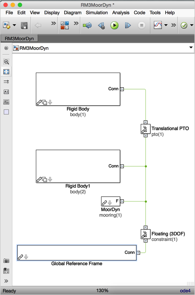
WEC-Sim Input File: In the
wecSimInputFile.mfile, the user needs to initiate the mooring class and MoorDyn and define the number of mooring lines.
%% Simulation Data
simu = simulationClass();
simu.simMechanicsFile = 'RM3MoorDyn.slx';       % WEC-Sim Model File
simu.mode = 'accelerator';
simu.explorer = 'off';
simu.rampTime = 40;
simu.endTime = 400;
simu.dt = 0.01;
simu.cicDt = 0.05;

%% Wave Information
% User-Defined Time-Series
waves = waveClass('elevationImport');           % Create the Wave Variable and Specify Type
waves.elevationFile = 'etaData.mat';            % Name of User-Defined Time-Series File [:,2] = [time, eta]
waves.waterDepth = 70;

%% Body Data
% Float
body(1) = bodyClass('../../_Common_Input_Files/RM3/hydroData/rm3.h5');
body(1).geometryFile = '../../_Common_Input_Files/RM3/geometry/float.stl';
body(1).mass = 'equilibrium';
body(1).inertia = [20907301 21306090.66 37085481.11];

% Spar/Plate
body(2) = bodyClass('../../_Common_Input_Files/RM3/hydroData/rm3.h5');
body(2).geometryFile = '../../_Common_Input_Files/RM3/geometry/plate.stl';
body(2).mass = 'equilibrium';
body(2).inertia = [94419614.57 94407091.24 28542224.82];
body(2).initial.displacement = [0 0 -0.21];     % Initial Displacement

%% PTO and Constraint Parameters
% Floating (3DOF) Joint
constraint(1) = constraintClass('Constraint1');
constraint(1).location = [0 0 0];

% Translational PTO
pto(1) = ptoClass('PTO1');
pto(1).stiffness=0;
pto(1).damping=1200000;
pto(1).location = [0 0 0];

%% Mooring
% Moordyn
mooring(1) = mooringClass('mooring');           % Initialize mooringClass
mooring(1).moorDyn = 1;                         % Initialize MoorDyn
mooring(1).moorDynLines = 6;                    % Specify number of lines
mooring(1).moorDynNodes(1:3) = 16;              % Specify number of nodes per line
mooring(1).moorDynNodes(4:6) = 6;               % Specify number of nodes per line
mooring(1).initial.displacement = [0 0 -21.29-.21]; % Initial Displacement (body cg + body initial displacement)
MoorDyn Input File: A mooring folder that includes a moorDyn input file (
lines.txt) is created. The moorDyn input file (lines.txt) is shown in the figure below. More details on how to set up the MooDyn input file are described in the MoorDyn Documentation. One specific requirement when using WEC-Sim with MoorDyn is that the Body(s) in which the mooring lines are attached to should be labeled as “Coupled” in the MoorDyn input file, which allows for WEC-Sim to control the body dynamics. Note: WEC-Sim now uses MoorDyn v2.
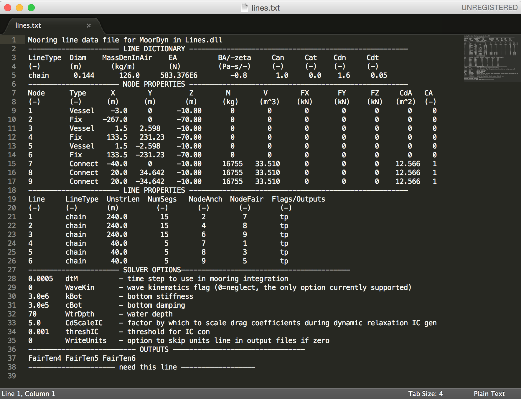
Simulation and Post-processing: Simulation and post-processing are the same process as described in Tutorial Section.
Note
You may need to install the MinGW-w64 compiler to run this simulation.
WEC-Sim Post-Processing
WEC-Sim contains several built in methods inside the response class and wave
class to assist users in processing WEC-Sim output: output.plotForces,
output.plotResponse, output.saveViz, waves.plotElevation, and
waves.plotSpectrum. This section will demonstrate the use of these methods.
They are fully documented in the WEC-Sim API.
Plot Forces
The responseClass.plotForces() method can be used to plot the time series of
each force component for a body. The first argument takes in a body number, the
second a degree of freedom of the force. For example, output.plotForces(2,3)
will plot the vertical forces that act on the 2nd body. The total force is split
into its components:
total force
excitation force
radiation damping force
added mass force
restoring force (combination of buoyancy, gravity and hydrostatic stiffness),
Morison element and viscous drag force
linear damping force
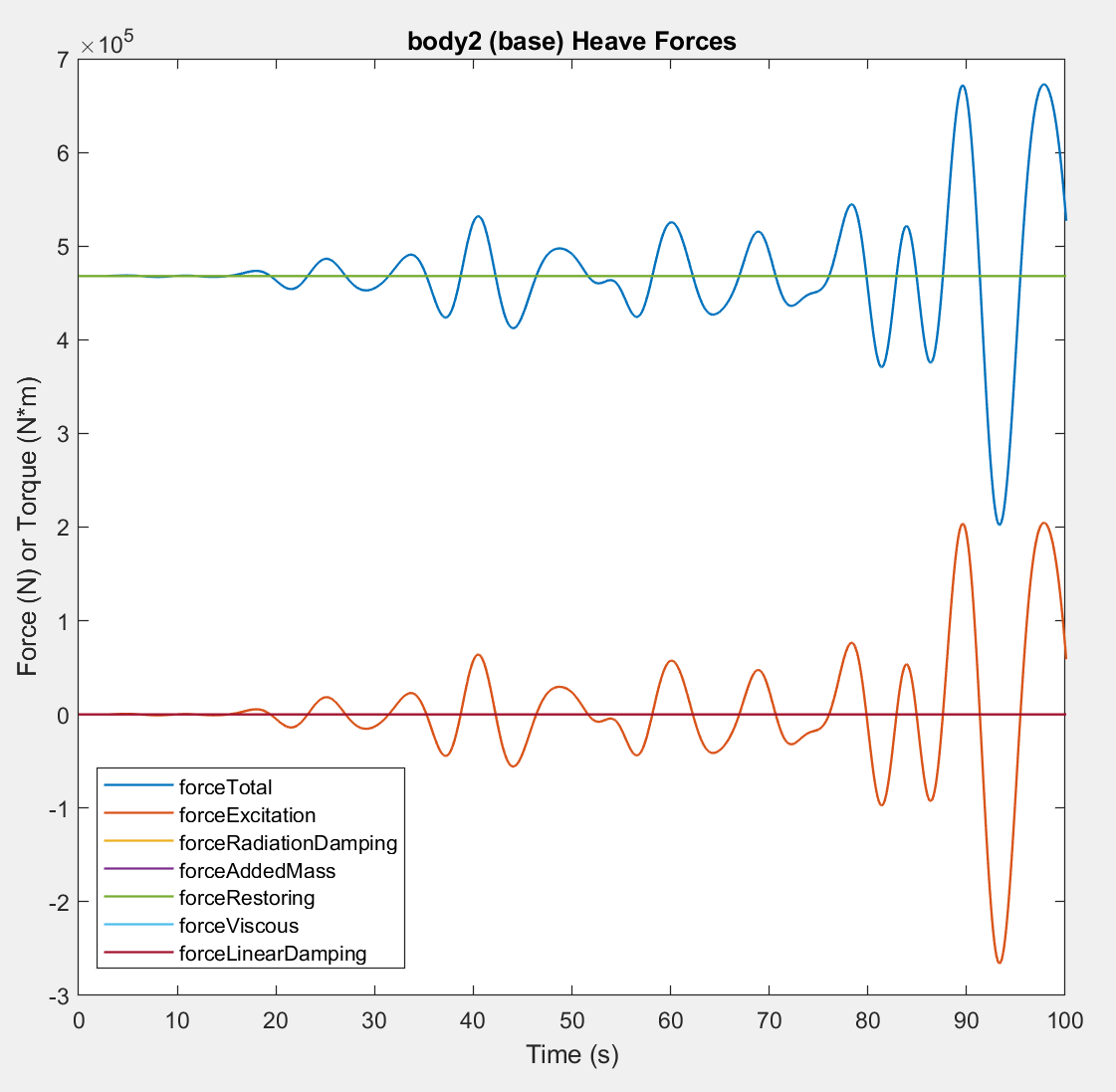
Demonstration of output.plotForces() method for the OSWEC example.
Plot Response
The responseClass.plotResponse() method is very similar to plotForces
except that it will plot the time series of a body’s motion in a given degree
of freedom. For example, output.plotResponse(1,5) will plot the pitch motion
of the 1st body. The position, velocity and acceleration of that body is shown.
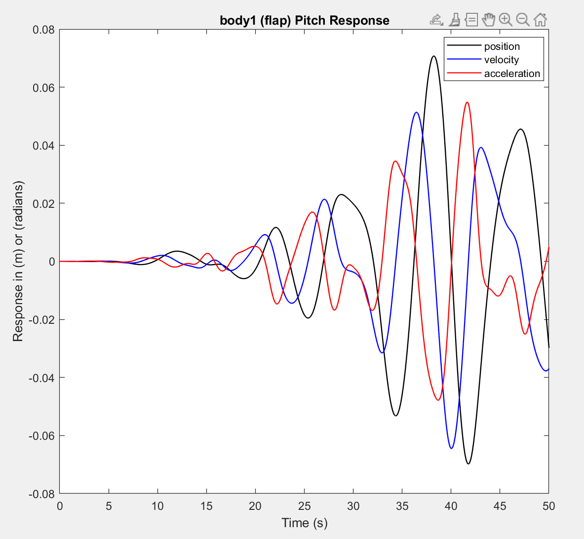
Demonstration of output.plotResponse() method for the OSWEC example.
Plot Elevation
The waveClass.plotElevation() method can be used to plot the wave elevation time
series at the domain origin. The ramp time is also marked. The only required input
is simu.rampTime. Users must manually plot or overlay the wave elevation at a
wave gauge location.
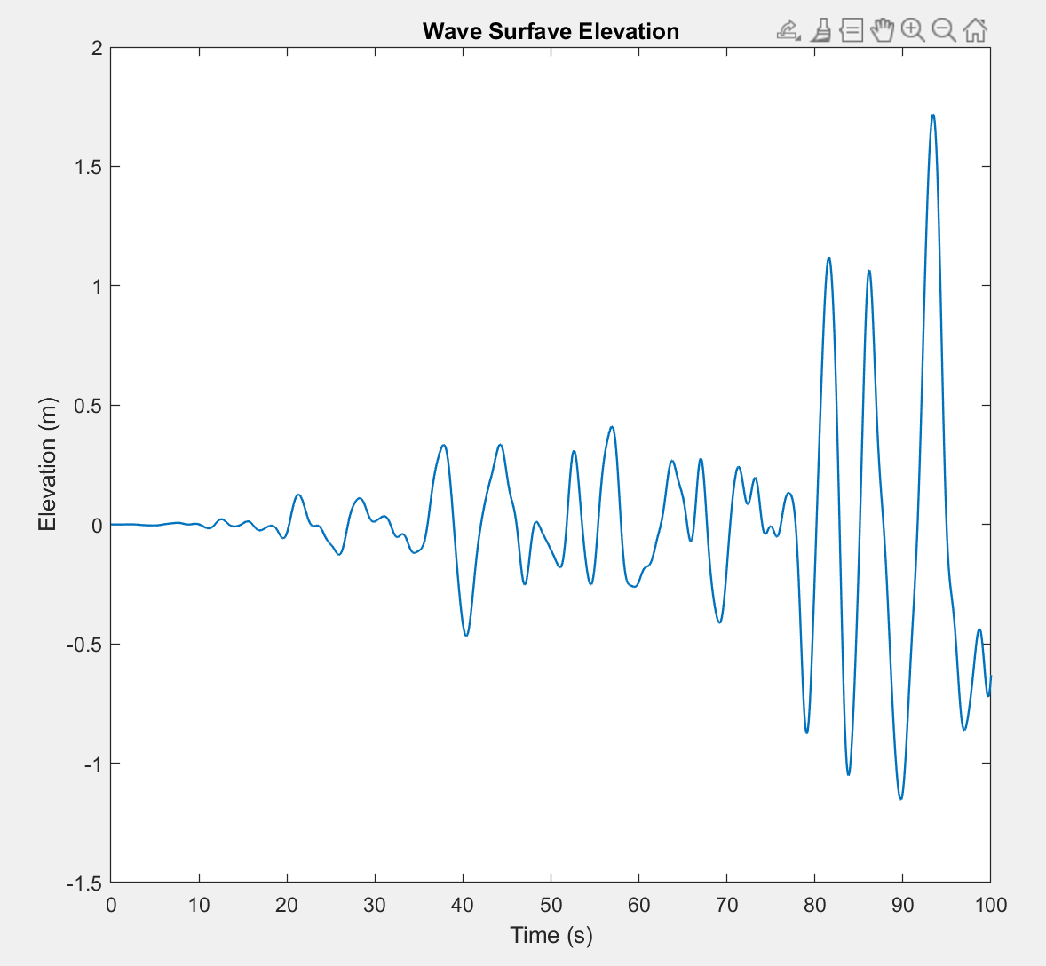
Demonstration of waves.plotElevation() method for the OSWEC example.
Plot Spectrum
The waveClass.plotSpectrum() method can be used to plot the frequency spectrum
of an irregular or spectrum import wave. No input parameters are required.
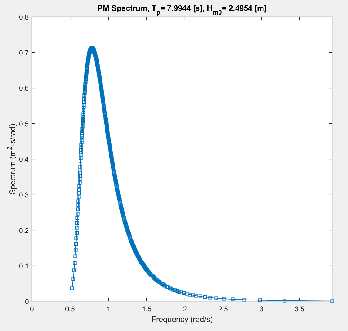
Demonstration of waves.plotSpectrum() method for the OSWEC example.
WEC-Sim Visualization
WEC-Sim provides visualization in SimScape Mechanics Explorer by default. This section describes some additional options for WEC-Sim visualization
Wave Markers
This section describes how to visualize the wave elevations at various locations using
markers in SimScape Mechanics Explorer.
Users must define an array of [X,Y] coordinates, the marker style (sphere, cube, frames), the marker size in pixels, marker color in RGB format.
The Global Reference Frame block programmatically initiates and adds/deletes the visualization blocks based on the number of markers (0 to N) defined by the user.
Here are the steps to define wave markers representing a wave-spectra, waves(1). Similar steps can be followed for subsequent waves(#) objects.
Define an array of marker locations:
waves(1).marker.location = [X,Y], where the first column defines the X coordinates, and the second column defines the corresponding Y coordinates, Default =[]Define marker style :
waves(1).marker.style = 1, where 1: Sphere, 2: Cube, 3: Frame, Default =1: SphereDefine marker size :
waves(1).marker.size = 10, to specify marker size in Pixels, Default =10Define marker color:
waves(1).marker.graphicColor = [1,0,0], to specifie marker color in RBG format.
For more information about using ParaView for visualization, refer to the Wave_Markers examples on the WEC-Sim Applications repository.
Note
This feature is not compatible with user-defined waves waves = waveClass('elevationImport')
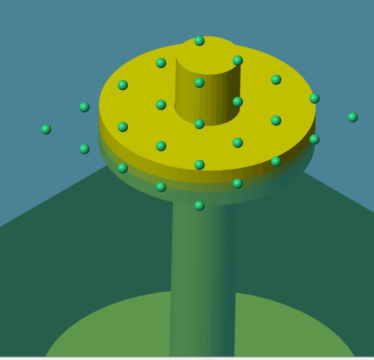
Demonstration of visualization markers in SimScape Mechanics Explorer.
Save Visualization
The responseClass.saveViz() method can be used to create a complete
animation of the simulation. The animation shows the 3D response of all bodies
over time on top of a surface plot of the entire directional wave field. The
default wave domain is defined by simu.domainSize, waves.waterDepth, and
the maximum height that the STL mesh of any body reaches. Users may optionally
input the axis limits to restrict or widen the field of view, the time steps per
animation frame, and the output file format. Users can choose to save the animation
as either a .gif or .avi file. This function can take significant time to
run depending on simulation time and time step, however it may be faster and easier
than Paraview. Users are still recommended to use the provided Paraview macros for
more complex animations and analysis.
For example, in the OSWEC case the command
output.saveViz(simu,body,waves,'timesPerFrame',5,'axisLimits',[-50 50 -50 50 -12 20])
results in the following figure:
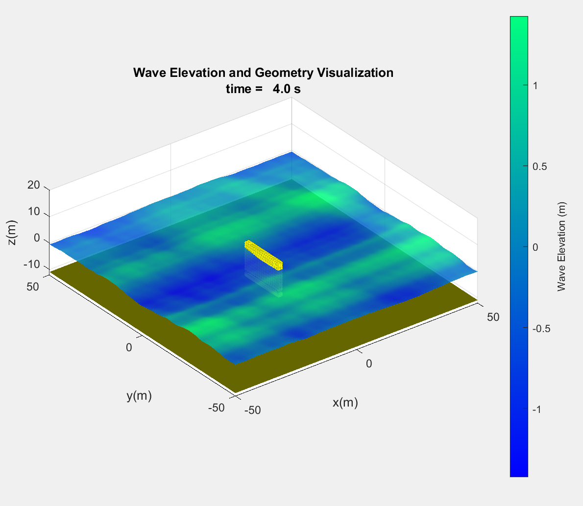
Demonstration of output.saveViz() method for the OSWEC example.
Paraview Visualization
This section describes how to use ParaView for visualizing data from a WEC-Sim simulation. Using ParaView visualization improves on the SimMechanics explorer by:
Visualizing the wave field
Visualizing the cell-by-cell nonlinear hydrodynamic forces (when using nonlinear buoyancy and Froude-Krylov wave excitation)
Allowing data manipulation and additional visualization options
However, the SimMechanics explorer shows the following information not included in the ParaView visualization:
Location of center of gravity
Location of different frames (e.g. PTO and Constraint frames)
Visualization with ParaView requires additional output files to be written to a vtk directory.
This makes the WEC-Sim simulation take more time and the case directory larger, so it should only be used when additional visualization is desired.
Users will also need to have some familiarity with using ParaView.
For more information about using ParaView for visualization, refer to the Series 4 - Body-to-Body Interactions, and the Paraview_Visualization examples on the WEC-Sim Applications repository.
Install ParaView and WEC-Sim Macros
First, install ParaView 5.11.1. Then, add the WEC-Sim specific macros:
Open ParaView
Click on
Macros => Add new macroNavigate to the WEC-Sim
source/functions/paraviewdirectorySelect the first file and click
OKRepeat this for all .py files in the
source/functions/paraviewdirectory
WEC-Sim Visualization in ParaView
When simu.paraview.option = 1, a vtk directory is created inside the WEC-Sim $CASE directory.
All files necessary for ParaView visualization are located there.
To view in ParaView:
Open the
$CASE/vtk/<filename>.pvdfile in ParaViewSelect the WEC-Sim model in the pipeline, and run the
WEC-SimmacroMove the camera to desired view
Click the green arrow (play) button
The WEC-Sim macro:
Extracts each body, sets the color and opacity, and renames them
Extracts the waves, sets color and opacity, and renames
Creates the ground plane
Sets the camera to top view
After opening the .pvd file and running the WEC-Sim macro you can do a number of things to visualize the simulation in different ways.
You can color waves and bodies by any of the available properties and apply any of the ParaView filters. The figures below show some of the visualization possibilities afforded by using ParaView with WEC-Sim.
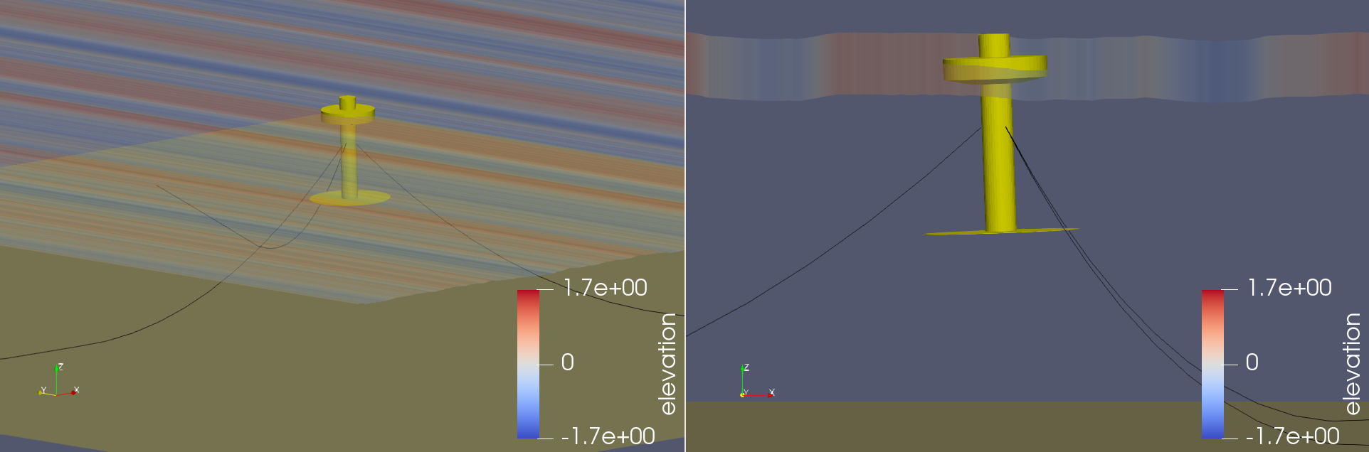
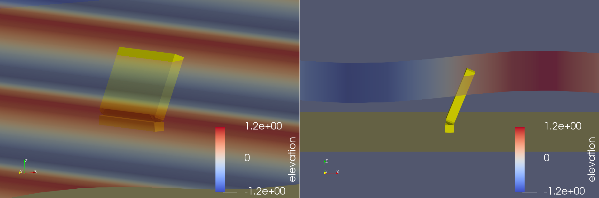
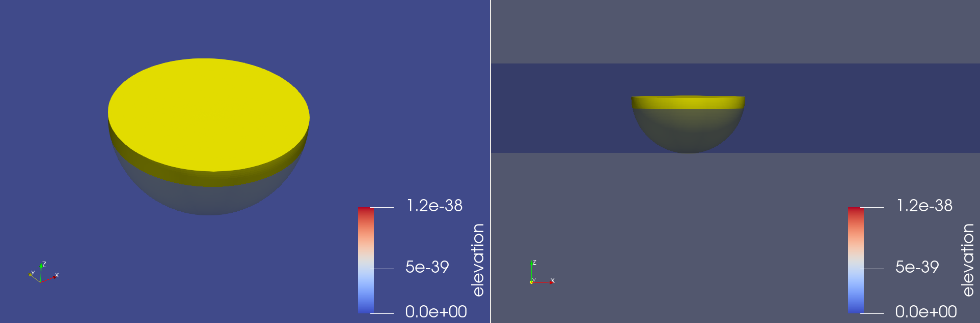
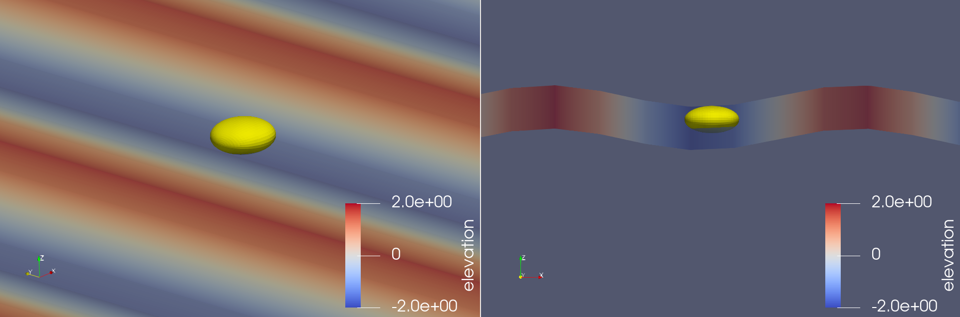
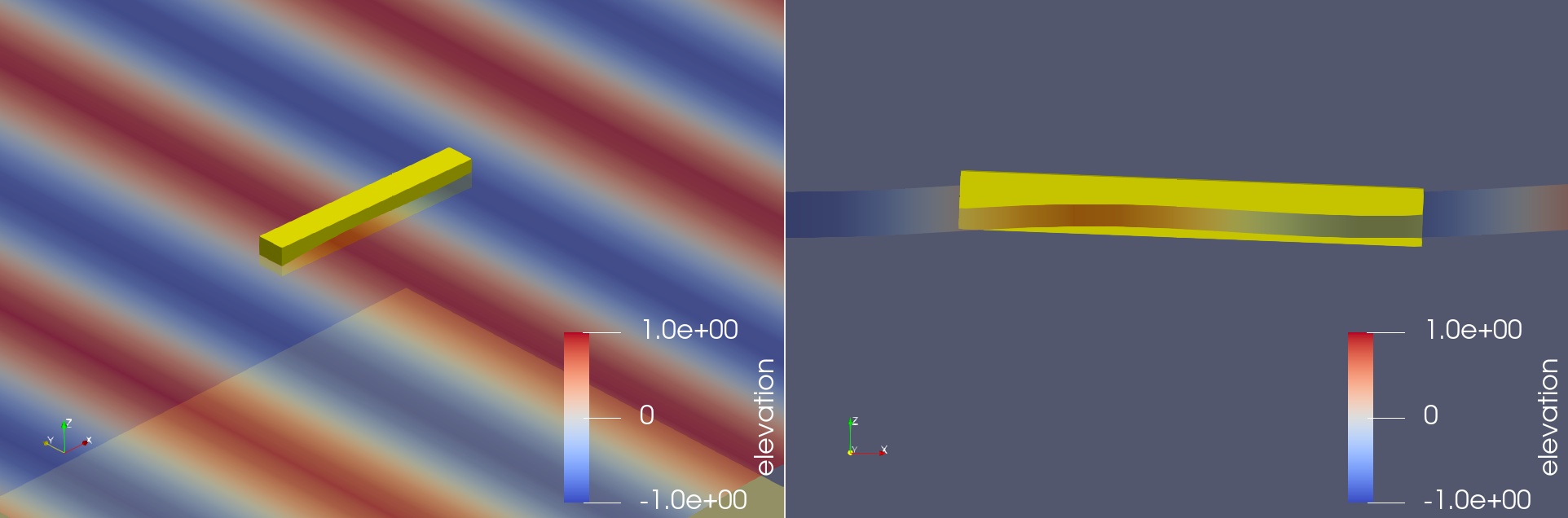
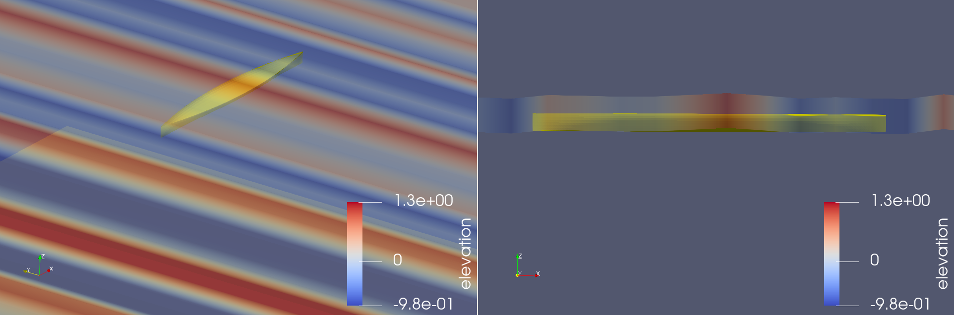
Wigley Ship Hull
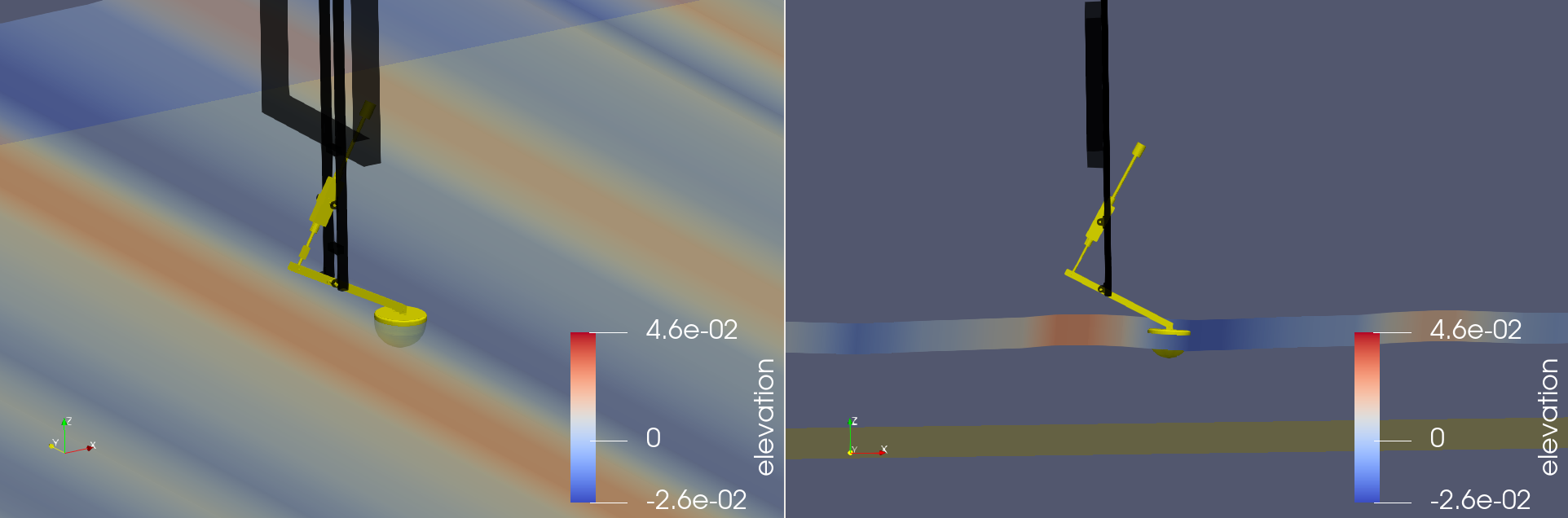
Wave Energy Converter Control Competition (WECCCOMP) Wavestar Device
OC6 Phase I DeepCwind Floating Semisubmersible
Two examples using Paraview for visualization of WEC-Sim data are provided in the Paraview_Visualization directory of the WEC-Sim Applications repository. The RM3_MoorDyn_Viz example uses ParaView for WEC-Sim data visualization of a WEC-Sim model coupled with MoorDyn to simulate a mooring system for the RM3 geometry. The OSWEC_NonLinear_Viz example uses ParaView for WEC-Sim data visualization of a WEC-Sim model with nonlinear Hydro to simulate nonlinear wave excitation on the flap of the OSWEC geometry.
MoorDyn Visualization in ParaView
The video below shows three different views of the RM3 model with MoorDyn.
The left view uses the WEC-Sim macro.
The top right view uses the slice filter.
The bottom right view shows the free surface colored by wave elevation.
Nonlinear Hydro Visualization in ParaView
When using nonlinear buoyancy and Froude-Krylov wave excitation the paraview files also contain cell data for the bodies. The cell data are:
Cell areas
Hydrostatic pressures
Linear Froude-Krylov pressures
Nonlinear Froude-Krylov pressures
The pressureGlyphs macro calculates cell normals, and cell centers. It then creates the following glyphs:
Hydrostatic pressure
Linear Froude-Krylov pressure
Nonlinear Froude-Krylov pressure
Total pressure (hydrostatic plus nonlinear Froude-Krylov)
Froude-Krylov delta (nonlinear minus linear)
To view WEC-Sim nonlinear hydro data in ParaView:
Open the
$CASE/vtk/<filename>.pvdfile in ParaViewSelect the WEC-Sim model in the pipeline, and run the
WEC-SimmacroMove the camera to desired view
Select the WEC-Sim model again in the pipeline, and run the
pressureGlyphsmacroSelect which features to visualize in the pipeline
Click the green arrow (play) button
The video below shows three different views of the OSWEC model with non-linear hydrodynamics. The top right shows glyphs of the nonlinear Froude-Krylov pressure acting on the float. The bottom right shows the device colored by hydrostatic pressure.
Loading a ParaView State File
If a previous *.pvsm ParaView state file was saved, the state can be applied to a *.pvd ParaView file. To load a state file:
Open the
$CASE/vtk/<filename>.pvdfile in ParaViewClick on
File => Load StateSelect the desired
$CASE/<filename>.pvsmParaview state file to applySelect the “Search files under specified directory” option, specify the desired WECS-Sim
$CASE/vtk/directory, and clickOK
Paraview state files are provided for both Paraview_Visualization examples provided onthe WEC-Sim Applications repository, one for the RM3 using MoorDyn, and another for the OSWEC with nonlinear hydro.
ParaView Visualization Parameters
The following table lists the WEC-Sim simulation parameters that can be specified in the wecSimInputFile to control the ParaView visualization. Note, the body.viz properties are also used for the SimMechanics explorer visualization.
WEC-Sim Visualization using ParaView |
||
|---|---|---|
Variable |
Description |
|
simu.paraview.option |
0 to not output ParaView files [default]
1 to output ParaView files
|
|
|
time (s) to start ParaView visualization |
|
|
time (s) to end ParaView visualization |
|
|
time step between adjacent ParaView frames [default 1] |
|
|
directory to create ParaView visualization files |
|
simu.nonlinearHydro |
0 for no nonlinear hydro [default]
1 for nonlinear hydro with mean free surface
2 for nonlinear hydro with instantaneous free surface
|
|
|
size of ground and water planes in meters [default 200] |
|
|
simulation output sampling time step [default dt] |
|
|
[RGB] body color [default [1 1 0]] |
|
|
body opacity [default 1] |
|
body(i).paraview |
0 to exclude body from ParaView visualization
1 to include body in ParaView visualization [default]
|
|
|
wave plane discretization: number of X points [default 50] |
|
|
||
Decay Tests
When performing simulations of decay tests, you must use one of the no-wave
cases and setup the initial (time = 0) location of each body, constraint, PTO,
and mooring block. The initial location of a body or mooring block is set by
specifying the centerGravity or location at the stability position (as with any WEC-Sim
simulation) and then specifying an initial displacement. To specify an initial
displacement, the body and mooring blocks have a .initial property
with which you can specify a translation and angular rotation about an
arbitrary axis. For the constraint and PTO blocks, the .location property
must be set to the location at time = 0.
There are methods available to help setup this initial displacement for all bodies, constraints, PTOs, and moorings. To do this, you would use the:
body(i).setInitDisp()constraint(i).setInitDisp()pto(i).setInitDisp()mooring(i).setInitDisp()
methods in the WEC-Sim input file. A description of the required input can be
found in the method’s header comments. The following properties must be
defined prior to using the object’s setInitDisp() method:
body(i).centerGravityconstraint(i).locationpto(i).locationmooring.location
For more information, refer to the Free Decay example on the WEC-Sim Applications repository.
Other Features
The WEC-Sim Applications repository also includes examples of using WEC-Sim to model a Desalination plant and a numerical model of the WaveStar device for control implementation. The WaveStar device was used in the WECCCOMP wave energy control competition.
References
Giorgio Bacelli and Ryan G Coe. Comments on control of wave energy converters. IEEE Transactions on Control Systems Technology, 29(1):478–481, 2020.
Giorgio Bacelli, Victor Nevarez, Ryan G Coe, and David G Wilson. Feedback resonating control for a wave energy converter. IEEE Transactions on Industry Applications, 56(2):1862–1868, 2019.
RPF Gomes, MFP Lopes, JCC Henriques, LMC Gato, and AFO Falcão. The dynamics and power extraction of bottom-hinged plate wave energy converters in regular and irregular waves. Ocean Engineering, 96:86–99, 2015.
Ryan G Coe, Giorgio Bacelli, and Dominic Forbush. A practical approach to wave energy modeling and control. Renewable and Sustainable Energy Reviews, 142:110791, 2021.
Aurélien Babarit and Alain H Clément. Optimal latching control of a wave energy device in regular and irregular waves. Applied Ocean Research, 28(2):77–91, 2006.
Ratanak So, Mike Starrett, Kelley Ruehl, and Ted KA Brekken. Development of control-sim: control strategies for power take-off integrated wave energy converter. In 2017 IEEE Power & Energy Society General Meeting, 1–5. IEEE, 2017.
Megaflux™ frameless direct drive torque motors. 2006. URL: https://www.alliedmotion.com/brushless-motors/brushless-direct-drive-torque-motors/megaflux-frameless-direct-drive-torque-motors/.