Tutorials

This section provides step-by-step instructions on how to set-up and run the WEC-Sim code using the provided Tutorials (located in the WEC-Sim $WECSIM/tutorials directory). Two WEC-Sim tutorials are provided: the Two-Body Point Absorber (RM3), and the Oscillating Surge WEC (OSWEC). For cases that are already set-up and ready to run, see Step 3 of Install WEC-Sim.

For information about the implementation of the WEC-Sim code refer to the Code Structure section. For information about additional WEC-Sim features, refer to Advanced Features.

Two-Body Point Absorber (RM3)

This section describes the application of the WEC-Sim code to model the Reference Model 3 (RM3) two-body point absorber WEC. This tutorial is provided in the WEC-Sim code release in the $WECSIM/tutorials directory.

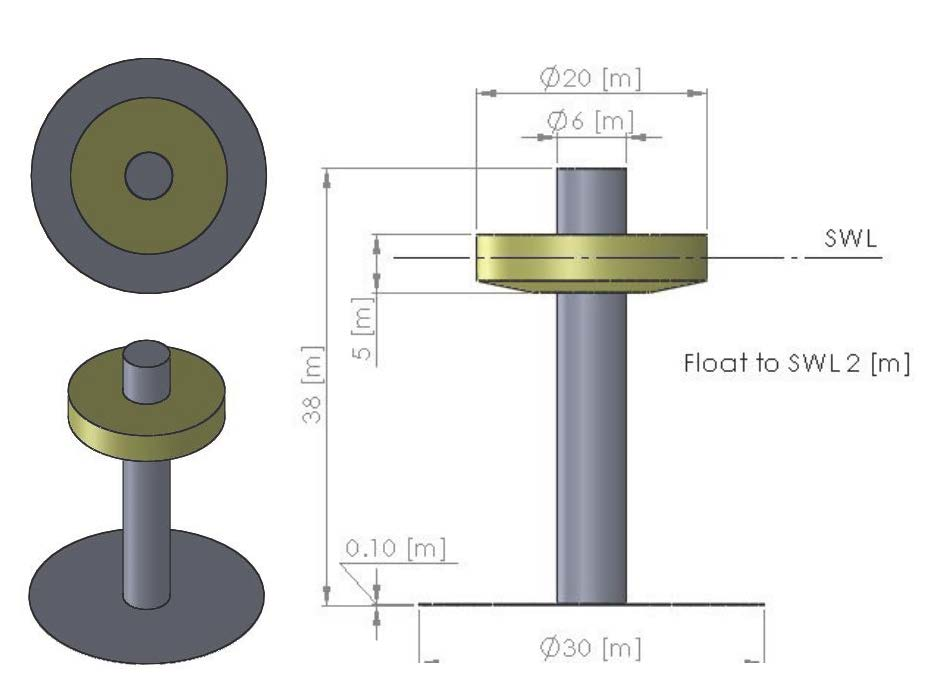
Device Geometry

The RM3 two-body point absorber WEC has been characterized both numerically and experimentally as a result of the DOE-funded Reference Model Project. The RM3 is a two-body point absorber consisting of a float and a reaction plate. Full-scale dimensions and mass properties of the RM3 are shown below.

Body	Mass (tonne)
Float	727.01
Plate	878.30

Body	Direction	Center of Gravity* (m)	Inertia Tensor (kg m^2)
Float	x	0	20,907,301	0	0
	y	0	0	21,306,091	0
	z	-0.72	0	0	37,085,481
Plate	x	0	94,419,615	0	0
	y	0	0	94,407,091	0
	z	-21.29	0	0	28,542,225

* The origin lies at the undisturbed free surface (SWL)

Model Files

Below is an overview of the files required to run the RM3 simulation in WEC-Sim. For the RM3 WEC, there are two corresponding geometry files: float.stl and plate.stl. In addition to the required files listed below, users may supply a userDefinedFunctions.m file for post-processing results once the WEC-Sim run is complete.

File Type	File Name	Directory
Input File	wecSimInputFile.m	$WECSIM/tutorials/rm3/
Simulink Model	rm3.slx	$WECSIM/tutorials/rm3/
Hydrodynamic Data	rm3.h5	$WECSIM/tutorials/rm3/hydroData/
Geometry Files	float.stl & plate.stl	$WECSIM/tutorials/rm3/geometry/

RM3 Tutorial

Step 1: Run BEMIO

Hydrodynamic data for each RM3 body must be parsed into a HDF5 file using BEMIO. BEMIO converts hydrodynamic data from WAMIT, NEMOH, Aqwa, or Capytaine into a HDF5 file, *.h5 that is then read by WEC-Sim. The RM3 tutorial includes data from a WAMIT run, rm3.out, of the RM3 geometry in the $WECSIM/tutorials/rm3/hydroData/ directory. The RM3 WAMIT rm3.out file and the BEMIO bemio.m script are then used to generate the rm3.h5 file.

This is done by navigating to the $WECSIM/tutorials/rm3/hydroData/ directory, and typing``bemio`` in the MATLAB Command Window:

>> bemio

Step 2: Build Simulink Model

The WEC-Sim Simulink model is created by dragging and dropping blocks from the WEC-Sim Library into the rm3.slx file. When setting up a WEC-Sim model, it is very important to note the base and follower frames. The base port should always connect ‘towards’ the Global Reference Frame, while the follower port connects ‘away’ from the reference frame. Also, a base port should always connect to a follower port. The same port type should not be connected (i.e. no base-base or follower-follower connections).

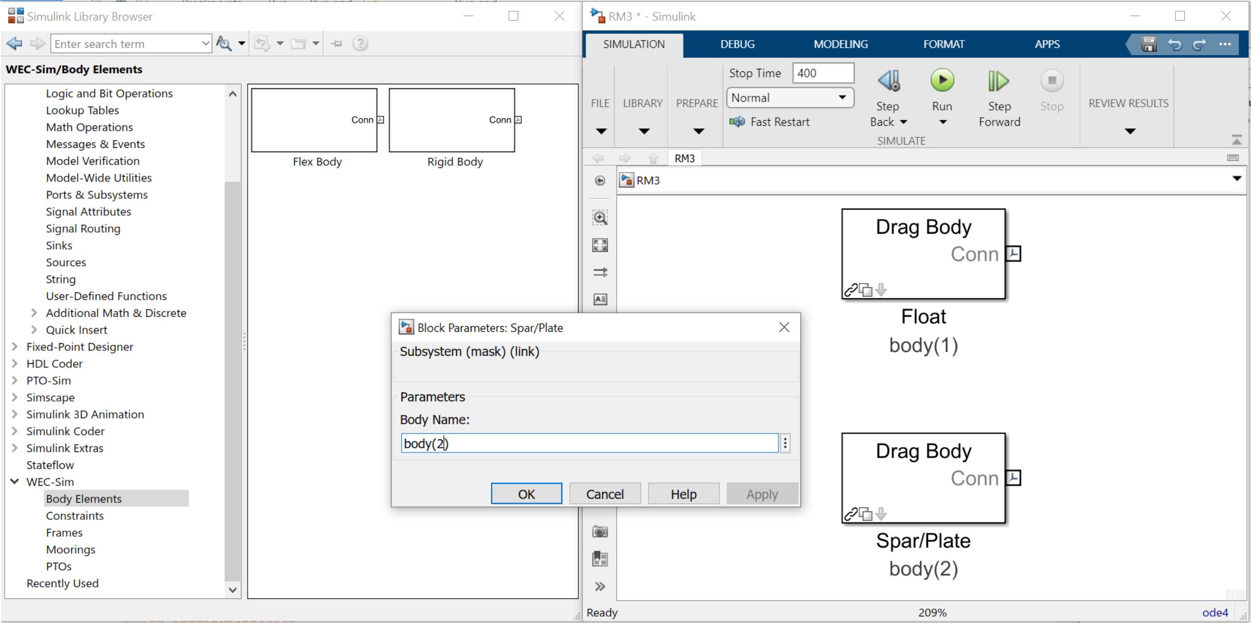
• Place two Rigid Body blocks from Body Elements in WEC-Sim Library in the Simulink model file, one for each RM3 rigid body.

• Double click on the Rigid Body block, and rename each instance of the body. The first body must be called body(1), and the second body should be called body(2).

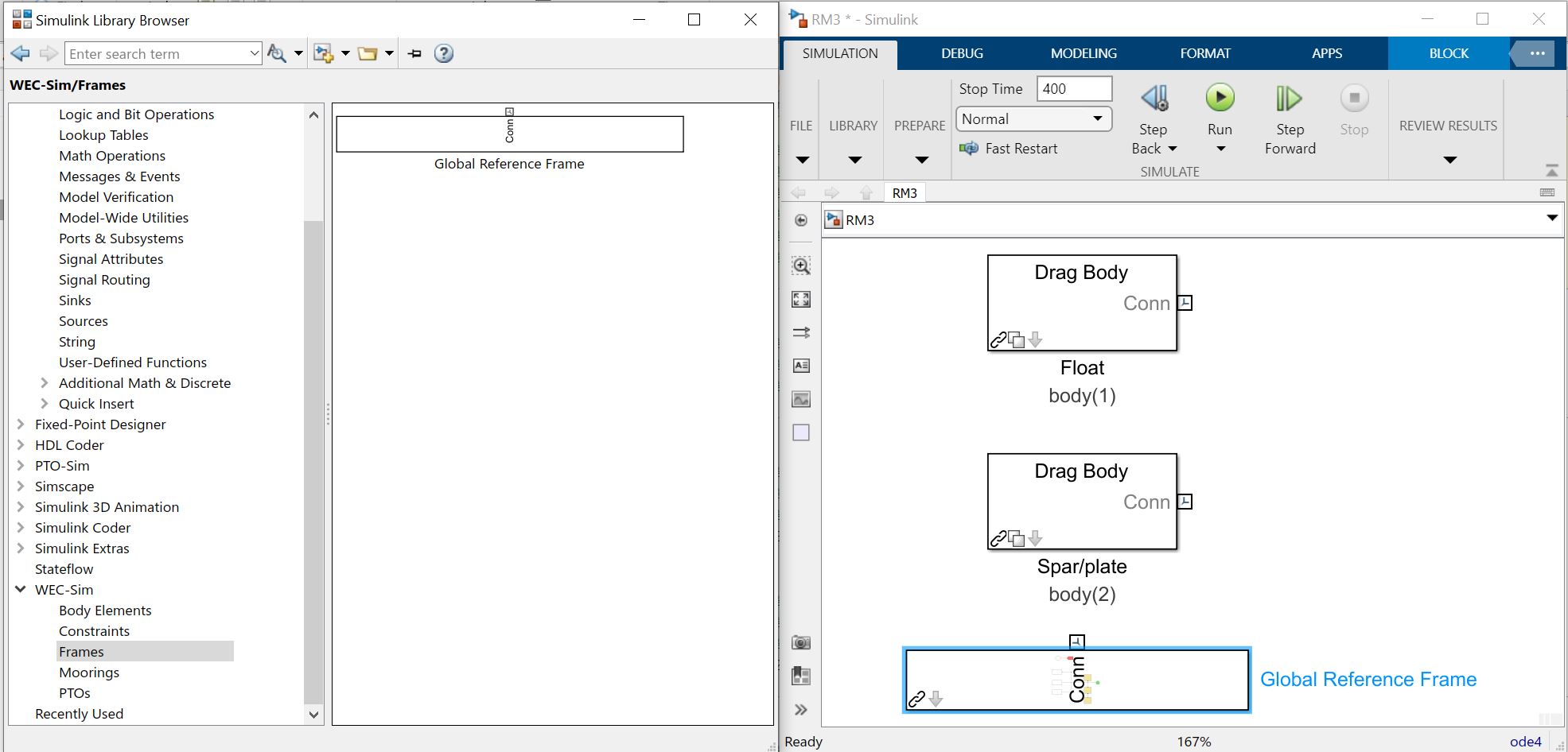
• Place the Global Reference Frame from Frames in the WEC-Sim Library in the Simulink model file. The global reference frame acts as the seabed.

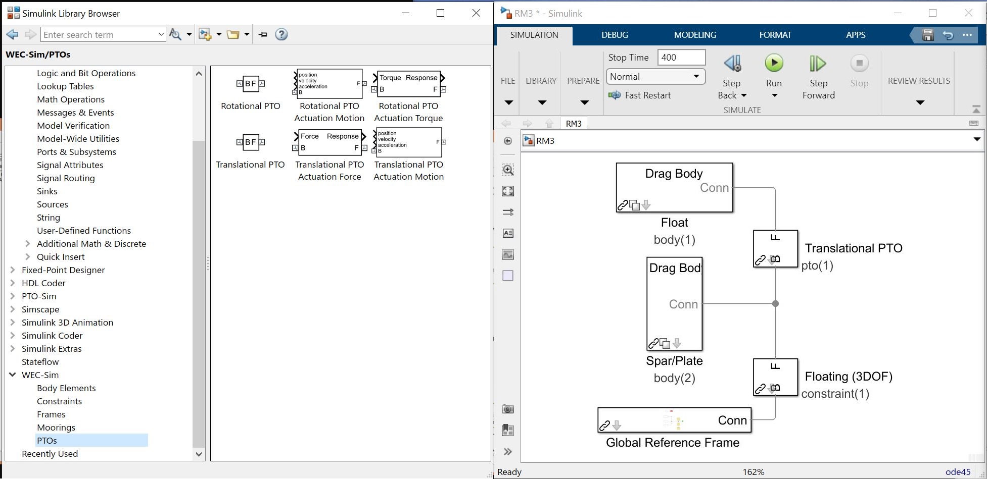
• Place the Floating (3DOF) block from Constrains to connect the plate to the seabed. This constrains the plate to move in 3DOF relative to the Global Reference Frame.

• Place the Translational PTO block from PTOs to connect the float to the spar. This constrains the float to move in heave relative to the spar, and allows definition of PTO damping.

Step 3: Write wecSimInputFile.m

The WEC-Sim input file defines simulation parameters, body properties, joints, and mooring for the RM3 model. The wecSimInputFile.m for the RM3 is provided in the RM3 case directory, and shown below.

New users should manually write the wecSimInputFile.m to become familiar with the set-up parameters and the files being called in a basic WEC-Sim run. First, define the simulation parameters. Initialize an instance of the simulationClass. Define the simulink file to use, the start, ramp and end times, and the time step required. The simulation class also controls all relevant numerical options and simulation-wide parameters in a single convenient class.

Next set-up the type of incoming wave by instantiating the waveClass. ‘Regular’ is a sinusoidal wave and the easiest to start with. Define an appropriate wave height and period. Waves can also be an irregular spectrum, imported by elevation or spectrum, or multidirectional.

Third, define all bodies, PTOs and constraints present in the simulink file. There are distinct classes for bodies, PTOs and constraints that contain different properties and function differently. Bodies are hydrodynamic and contain mass and geometry properties. Initialize bodies by calling the bodyClass and the path to the relevant h5 file. Set the path to the geometry file, and define the body’s mass properties. PTOs and constraints are more simple and contain forces and power dissipation (in the constraint) that limit the WEC’s motion. PTOs and constraints can be set by calling the appropriate class with the Simulink block name. Set the location and any PTO damping or stiffness desired.

%% Simulation Data
simu = simulationClass();                       % Initialize simulationClass
simu.simMechanicsFile = 'RM3.slx';              % Simulink Model File
simu.startTime = 0;                             % Simulation Start Time [s]
simu.rampTime = 100;                         	% Wave Ramp Time [s]
simu.endTime=400;                               % Simulation End Time [s]
simu.dt = 0.1;                                  % Simulation time-step [s]

%% Wave Information  
% Regular Waves 
waves = waveClass('regular');                   % Initialize waveClass
waves.height = 2.5;                                  % Wave Height [m]
waves.period = 8;                                    % Wave Period [s]

%% Body Data
% Float
body(1) = bodyClass('hydroData/rm3.h5');        % Initialize bodyClass for Float
body(1).geometryFile = 'geometry/float.stl';    % Geometry File
body(1).mass = 'equilibrium';                   % Mass [kg]
body(1).inertia = [20907301 21306090.66 37085481.11];  % Moment of Inertia [kg*m^2]     

% Spar/Plate
body(2) = bodyClass('hydroData/rm3.h5');        % Initialize bodyClass for Spar
body(2).geometryFile = 'geometry/plate.stl';    % Geometry File
body(2).mass = 'equilibrium';                   % Mass [kg]
body(2).inertia = [94419614.57 94407091.24 28542224.82]; % Moment of Inertia [kg*m^2]

%% PTO and Constraint Parameters
% Floating (3DOF) Joint
constraint(1) = constraintClass('Constraint1'); % Initialize constraintClass for Constraint1
constraint(1).location = [0 0 0];                    % Constraint Location [m]

% Translational PTO
pto(1) = ptoClass('PTO1');                      % Initialize ptoClass for PTO1
pto(1).stiffness = 0;                                   % PTO Stiffness [N/m]
pto(1).damping = 1200000;                             % PTO Damping [N/(m/s)]
pto(1).location = [0 0 0];                           % PTO Location [m]

Step 4: Run WEC-Sim

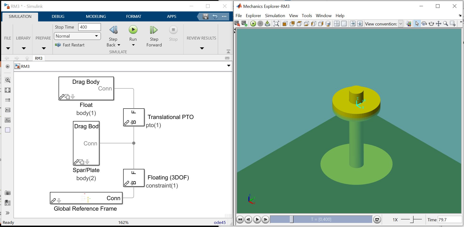
To execute the WEC-Sim code for the RM3 tutorial, type wecSim into the MATLAB Command Window. Below is a figure showing the final RM3 Simulink model and the WEC-Sim GUI during the simulation. For more information on using WEC-Sim to model the RM3 device, refer to [A1].

Step 5: Post-processing

The RM3 tutorial includes a userDefinedFunctions.m which plots RM3 forces and responses. This file can be modified by users for post-processing. Additionally, once the WEC-Sim run is complete, the WEC-Sim results are saved to the output variable in the MATLAB workspace.

Oscillating Surge WEC (OSWEC)

This section describes the application of the WEC-Sim code to model the Oscillating Surge WEC (OSWEC). This tutorial is provided in the WEC-Sim code release in the $WECSIM/tutorials directory.

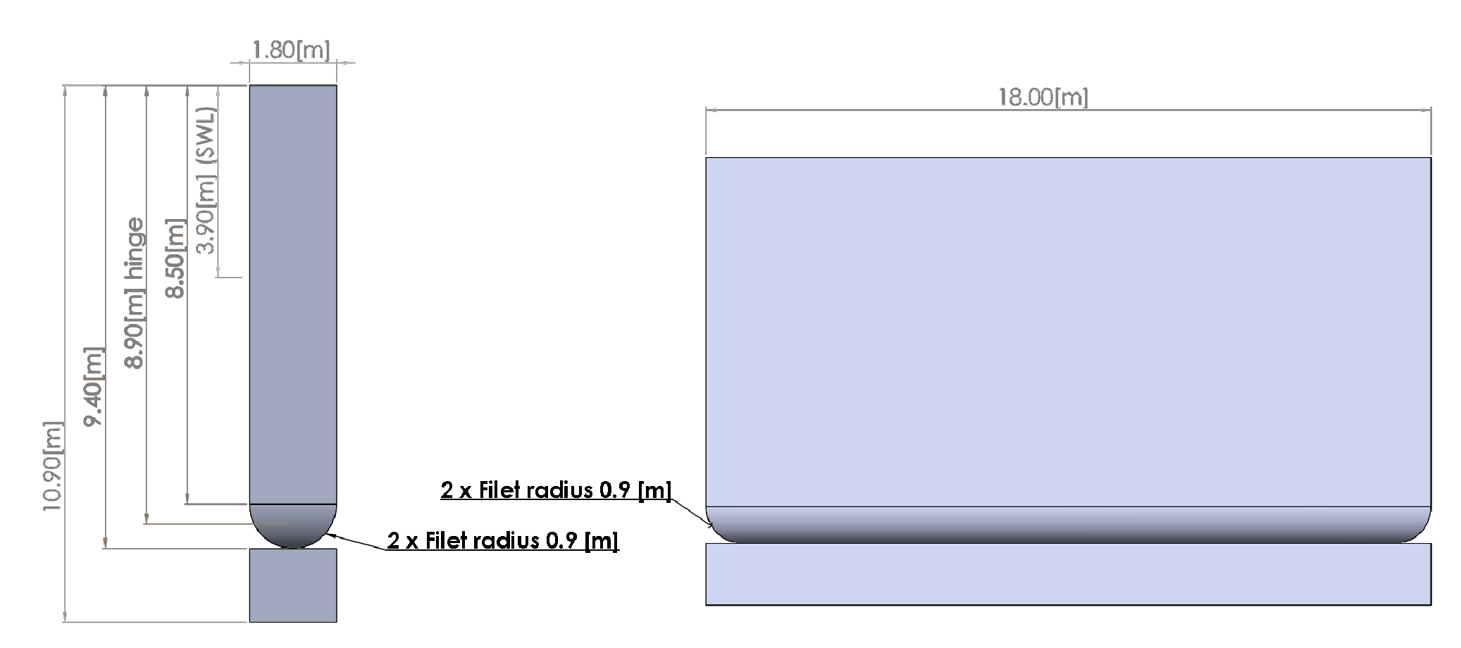
Device Geometry

The OSWEC was selected because its design is fundamentally different from the RM3. This is critical because WECs span an extensive design space, and it is important to model devices in WEC-Sim that operate under different principles. The OSWEC is fixed to the ground and has a flap that is connected through a hinge to the base that restricts the flap in order to pitch about the hinge. The full-scale dimensions and mass properties of the OSWEC are shown below.

Body	Mass (tonne)
Flap	127

Body	Direction	Center of Gravity* (m)	Moment of Inertia Tensor (kg m^2)
Flap	x	0	0	0	0
	y	0	0	1,850,000	0
	z	-3.9	0	0	0

Note

The global frame lies at the undisturbed free surface. The body-fixed frame is at the center of gravity. Since the OSWEC is modeled as a pitch device, only the Iyy Moment of Inertia has been defined.

Model Files

Below is an overview of the files required to run the OSWEC simulation in WEC-Sim. For the OSWEC, there are two corresponding geometry files: flap.stl and base.stl. In addition to the required files listed below, users may supply a userDefinedFunctions.m file for post-processing results once the WEC-Sim run is complete.

File Type	File Name	Directory
Input File	wecSimInputFile.m	$WECSIM/tutorials/oswec/
Simulink Model	oswec.slx	$WECSIM/tutorials/oswec/
Hydrodynamic Data	oswec.h5	$WECSIM/tutorials/oswec/hydroData/
Geometry Files	flap.stl & base.stl	$WECSIM/tutorials/oswec/geometry/

OSWEC Tutorial

Step 1: Run BEMIO

Hydrodynamic data for each OSWEC body must be parsed into a HDF5 file using BEMIO. BEMIO converts hydrodynamic data from WAMIT, NEMOH, Aqwa, or Capytaine into a HDF5 file, *.h5 that is then read by WEC-Sim. The OSWEC tutorial includes data from a WAMIT run, oswec.out, of the OSWEC geometry in the $WECSIM/tutorials/rm3/hydroData/ directory. The OSWEC WAMIT oswec.out file and the BEMIO bemio.m script are then used to generate the oswec.h5 file.

This is done by navigating to the $WECSIM/tutorials/oswec/hydroData/ directory, and typing``bemio`` in the MATLAB Command Window:

>> bemio

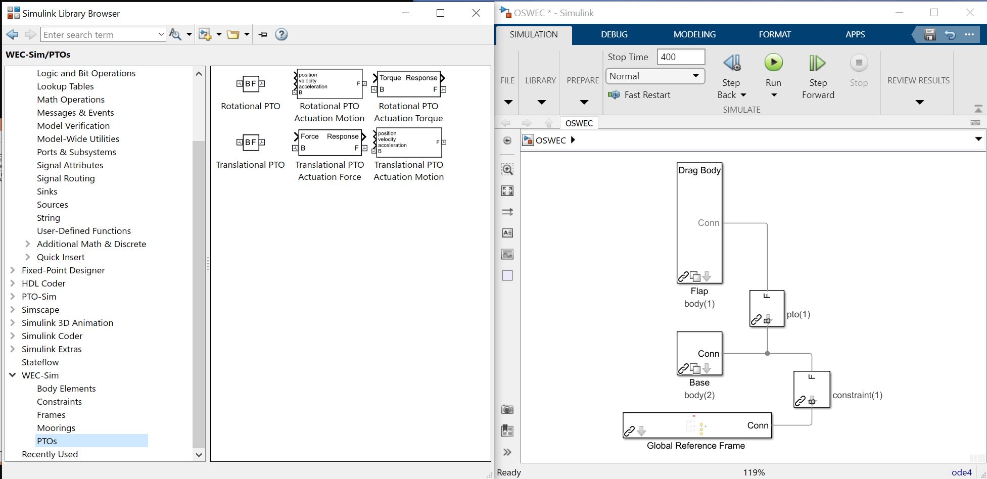
Step 2: Build Simulink Model

The WEC-Sim Simulink model is created by dragging and dropping blocks from the WEC-Sim Library into the oswec.slx file.

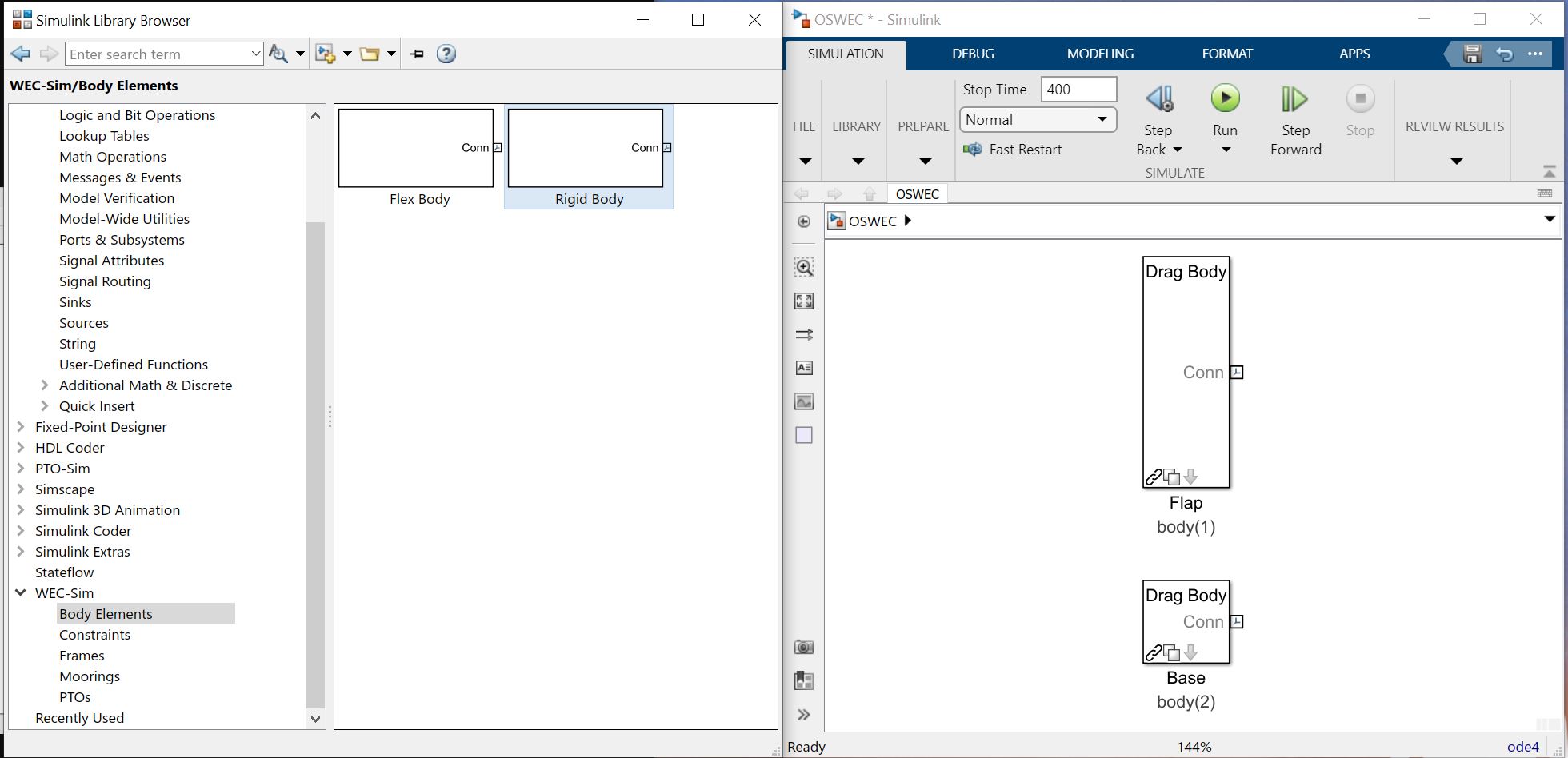
• Place two Rigid Body blocks from the WEC-Sim Library in the Simulink model file, one for each OSWEC rigid body.

• Double click on the Rigid Body block, and rename each instance of the body. The first body must be called body(1), and the second body should be called body(2).

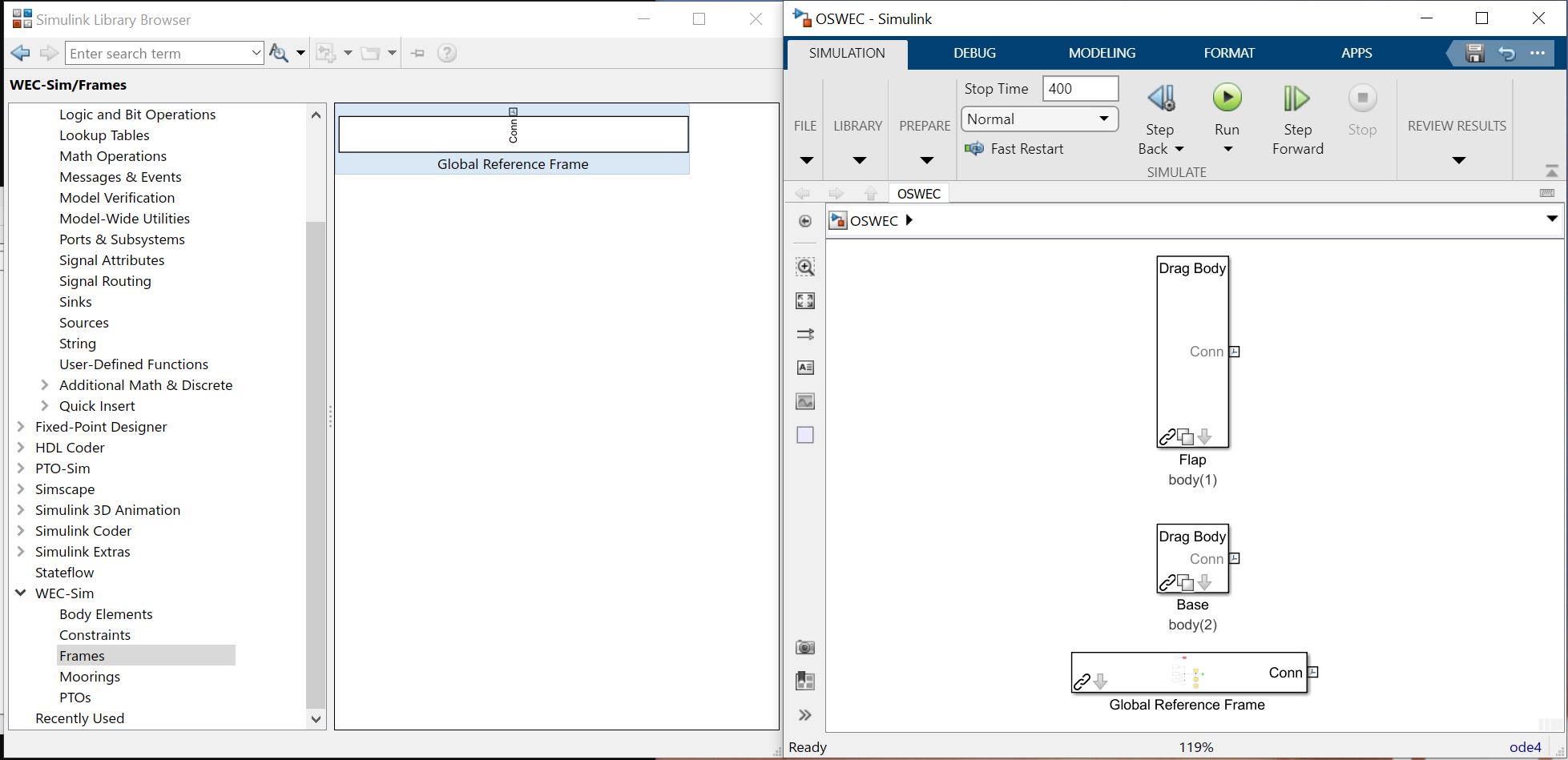
• Place the Global Reference Frame from Frames in the WEC-Sim Library in the Simulink model file. The global reference frame acts as the seabed.

• Place the Fixed block from Constraints to connect the base to the seabed. This constrains the base to be fixed relative to the Global Reference Frame.

• Place a Rotational PTO block to connect the base to the flap. This constrains the flap to move in pitch relative to the base, and allows for the definition of PTO damping.

Note

When setting up a WEC-Sim model, it is very important to note the base and follower frames.

Step 3: Write wecSimInputFile.m

The WEC-Sim input file defines simulation parameters, body properties, and joints for the OSWEC model. Writing the OSWEC input file is similar to writing the RM3 input. Try writing it on your own. Define the simulation class, wave class, bodies, constraints and PTOs. The wecSimInputFile.m for the OSWEC is provided in the OSWEC case directory, and shown below.

%% Simulation Data
simu = simulationClass();                       % Initialize simulationClass
simu.simMechanicsFile = 'OSWEC.slx';            % Simulink Model File
simu.startTime = 0;                             % Simulation Start Time [s]
simu.rampTime = 100;                            % Wave Ramp Time [s]
simu.endTime=400;                               % Simulation End Time [s]   
simu.dt = 0.1;                                  % Simulation Time-Step [s]

%% Wave Information
% Regular Waves 
waves = waveClass('regular');                   % Initialize waveClass                                 
waves.height = 2.5;                                  % Wave Height [m]
waves.period = 8;                                    % Wave Period [s]

%% Body Data
% Flap
body(1) = bodyClass('hydroData/oswec.h5');      % Initialize bodyClass for Flap 
body(1).geometryFile = 'geometry/flap.stl';     % Geometry File
body(1).mass = 127000;                          % Mass [kg]
body(1).inertia = [1.85e6 1.85e6 1.85e6];  % Moment of Inertia [kg-m^2]

% Base
body(2) = bodyClass('hydroData/oswec.h5');      % Initialize bodyClass for Base
body(2).geometryFile = 'geometry/base.stl';     % Geometry File
body(2).mass = 999;                             % Fixed Body Mass
body(2).inertia = [999 999 999];                % Fixed Body Inertia

%% PTO and Constraint Parameters
% Fixed
constraint(1)= constraintClass('Constraint1');  % Initialize constraintClass for Constraint1
constraint(1).location = [0 0 -10];                  % Constraint Location [m]

% Rotational PTO
pto(1) = ptoClass('PTO1');                      % Initialize ptoClass for PTO1
pto(1).stiffness = 0;                           % PTO Stiffness [Nm/rad]
pto(1).damping = 0;                                   % PTO Damping [Nsm/rad]
pto(1).location = [0 0 -8.9];                        % PTO Location [m]

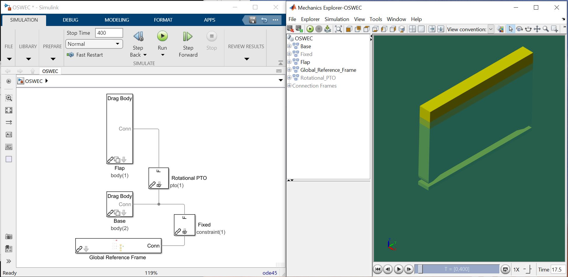
Step 4: Run WEC-Sim

To execute the WEC-Sim code for the OSWEC tutorial, type wecSim into the MATLAB Command Window. Below is a figure showing the final OSWEC Simulink model and the WEC-Sim GUI during the simulation. For more information on using WEC-Sim to model the OSWEC device, refer to [A2, A3].

Step 5: Post-processing

The OSWEC tutorial includes a userDefinedFunctions.m which plots OSWEC forces and responses. This file can be modified by users for post-processing. Additionally, once the WEC-Sim run is complete, the WEC-Sim results are saved to the output variable in the MATLAB workspace.

WEC-Sim Examples

Working examples of using WEC-Sim to model the RM3, OSWEC, and RM3FromSimulink are provided in the $WECSIM/examples/ directory. For each example the wecSimInputFile.m provided includes examples of how to run different wave cases:

• noWaveCIC - no wave with convolution integral calculation

• regularCIC - regular waves with convolution integral calculation

• irregular - irregular waves using a Pierson-Moskowitz spectrum with convolution integral calculation

• irregular - irregular waves using a Bretschneider Spectrum with state space calculation

• spectrumImport - irregular waves using a user-defined spectrum

• elevationImport - user-defined time-series

• Run from MATLAB Command Window (for RM3 and OSWEC examples)

  • Type wecSim in the Command Window

• Run from Simulink (for RM3FromSimulink example)

  • Open the relevant WEC-Sim Simulink file

  • Type initializeWecSim in the Command Window

  • Hit Play in Simulink model to run

To customize or develop a new WEC-Sim model that runs from Simulink (e.g. for Hardware-in-the-Loop, HIL, applications) refer to Running from Simulink for more information. Users may also use wecSimMCR, wecSimPCT, wecSimFcn and as described in the advanced features sections Multiple Condition Runs (MCR) and Parallel Computing Toolbox (PCT). These options are only available through the MATLAB Command Window.

References

[A1]

K. Ruehl, C. Michelen, S. Kanner, M. Lawson, and Y. Yu. Preliminary Verification and Validation of WEC-Sim, an Open-Source Wave Energy Converter Design Tool. In Proceedings of OMAE 2014. San Francisco, CA, 2014.

[A2]

Y. Yu, M. Lawson, K. Ruehl, and C. Michelen. Development and Demonstration of the WEC-Sim Wave Energy Converter Simulation Tool. In Proceedings of the 2nd Marine Energy Technology Symposium. Seattle, WA, USA, 2014.

[A3]

Y. Yu, Y. Li, K. Hallett, and C. Hotimsky. Design and Analysis for a Floating Oscillating Surge Wave Energy Converter. In Proceedings of OMAE 2014. San Francisco, CA, 2014.