Code Structure
This section provides a description of the WEC-Sim source code and its structure. For more information about WEC-Sim’s code structure, refer to the Code Structure webinar.
WEC-Sim Source Code
The directory where the WEC-Sim code is contained is referred to as $WECSIM
(e.g. C:/User/Documents/GitHub/WEC-Sim). The WEC-Sim source code files are
contained within a source directory referred to as $WECSIM/source. The
WEC-Sim source code consists primarily of three components as described in the table:
File Type |
File name |
Directory |
WEC-Sim Executable |
|
|
WEC-Sim MATLAB Functions |
|
|
WEC-Sim MATLAB Classes |
|
|
WEC-Sim Simulink Library |
|
|
The WEC-Sim executable is the wecSim.m file.
Executing wecSim from a case directory parses the user input data,
performs pre-processing calculations in each of the classes, selects and
initializes variant subsystems in the Simulink model, runs the time-domain
simulations in WEC-Sim, and calls post-processing scripts.
When a WEC-Sim case is properly set-up, the user only needs to use the single command wecSim
in the command line to run the simulation.
Users can run WEC-Sim from the command line with the command wecSim or from directly from Simulink,
refer to Running from Simulink.
WEC-Sim Classes
All information required to run WEC-Sim simulations is contained within the
simu, waves, body(i), constraint(i), pto(i), cable(i), and
mooring(i) objects (instances of the simulationClass, waveClass, bodyClass,
constraintClass, ptoClass, cableClass, and mooringClass).
Users can instantiate and interact with these classes within the WEC-Sim input
file (wecSimInputFile.m). The following Source Details
section describes the role of the WEC-Sim objects, and how to and interact with the
WEC-Sim objects to define input properties.
There are two ways to look at the available properties and methods within a
class. The first is to type doc <className> in Matlab Command Window, and
the second is to open the class definitions located in the
$WECSIM/source/objects directory by typing open <className> in MATLAB
Command Window. The latter provides more information since it also defines the
different fields in a structure.
WEC-Sim Library
In addition to the wecSimInputFile.m that instantiates classes, a WEC-Sim
simulation requires a simulink model (*.slx) that represents the WEC
system components and their connectivity. Similar to how the input file uses the
WEC-Sim classes, the Simulink model uses WEC-Sim library blocks. There should
be a one-to-one relationship between the objects defined in the input file and
the blocks used in the Simulink model.
The WEC-Sim library is divided different types of library blocks. Users should be able to model their WEC device using the available WEC-Sim blocks (and possibly other Simulink/Simscape blocks). The image below shows the WEC-Sim block grouping by type.
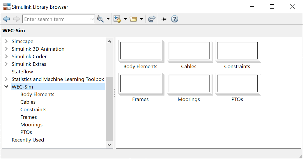
The following sections describe the different library types, the related class, and their general purpose.
Source Details
The WEC-Sim Classes and Library Blocks interact with one another during a simulation. The classes contain functions for initialization, reading input data, pre-processing and post-processing. The library blocks use these pre-processed parameters during the time-domain simulation in Simulink. The relationship between WEC-Sim Classes and their corresponding Library Blocks are described in the following sections, and summarized in the table below.
WEC-Sim Classes |
Corresponding Library Blocks |
Simulation Class and Wave Class |
Frames |
Body Class |
Body Elements |
Constraint Class |
Constraints |
PTO Class |
PTOs |
Cable Class |
Cables |
Mooring Class |
Moorings |
Simulation Class
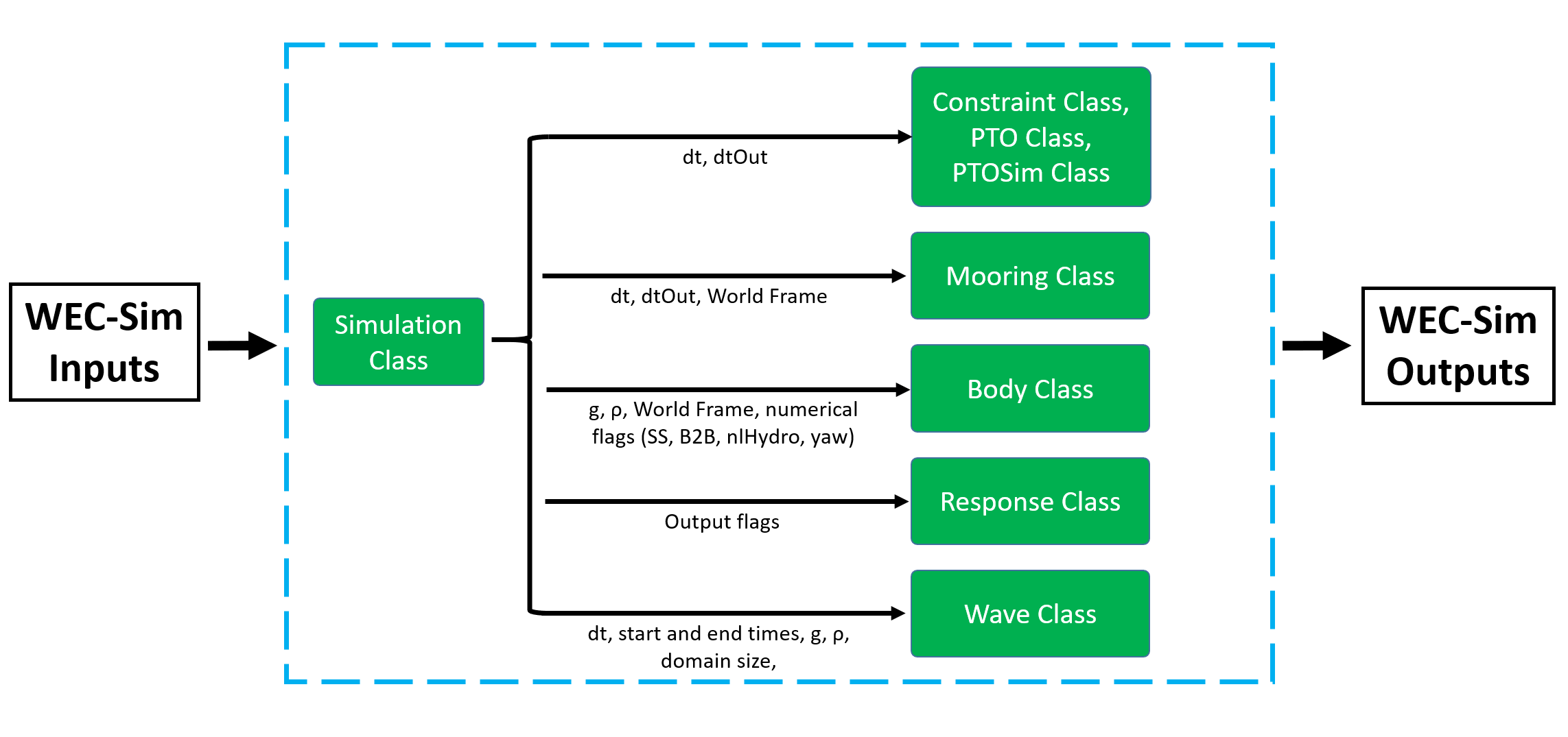
The simulation class contains the simulation parameters, flags and solver settings necessary to execute the WEC-Sim code. These simulation parameters include numerical settings such as the time step, start time, differential equation solver method, and flags for various output options and nonlinear hydrodynamics options. At a high level, the simulation class interacts with the rest of WEC-Sim as shown in the diagram below. The most common flags and attributes that are passed to other objects are the start, end, and ramp times, time steps, global variables (gravity, density, etc).
Simulation Class Initialization
Within the wecSimInputFile.m, users
must initialize the simulation class (simulationClass) and specify the name
of the WEC-Sim (*.slx) model file by including the following lines:
simu=simulationClass();
simu.simMechanicsFile='<modelFile>.slx'
All simulation class properties are specified as variables within the simu
object as members of the simulationClass.
The WEC-Sim code has default values defined for the simulation class
properties. These default values can be overwritten by the user in the input file,
for example, the end time of a simulation can be set by entering the following command:
simu.endTime = <user specified end time>.
Users may specify other simulation class properties using the simu object
in the wecSimInputFile.m, such as:
Simulation start time |
|
End time |
|
Ramp time |
|
Time step |
|
Available simulation properties, default values, and functions can be found by
typing doc simulationClass in the MATLAB command window, or by opening the
simulationClass.m file in $WECSIM/source/objects directory by typing open
simulationClass in MATLAB Command Window.
For more information about application of WEC-Sim’s simulation class, refer to
Simulation Features.
Frame Block
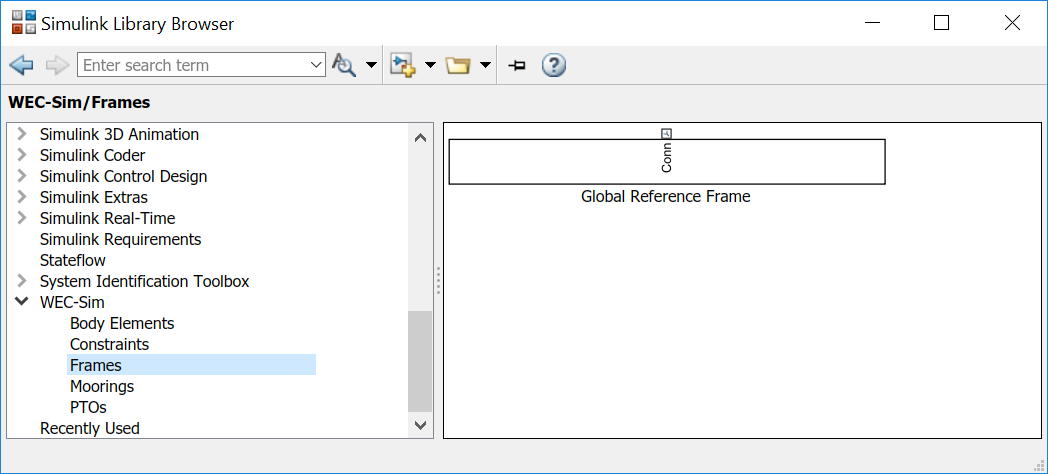
The simulation class is tied to the Frames library.
The Frames library contains one block that is necessary in every model. The
Global Reference Frame block defines the global coordinates, solver
configuration, seabed and free surface description, simulation time, and other
global settings. It can be useful to think of the Global Reference Frame as
being the seabed when creating a model. Every model requires one instance of
the Global Reference Frame block. The Global Reference Frame block uses the
simulation class variable simu and the wave class variable waves, which
must be defined in the input file.
Wave Class
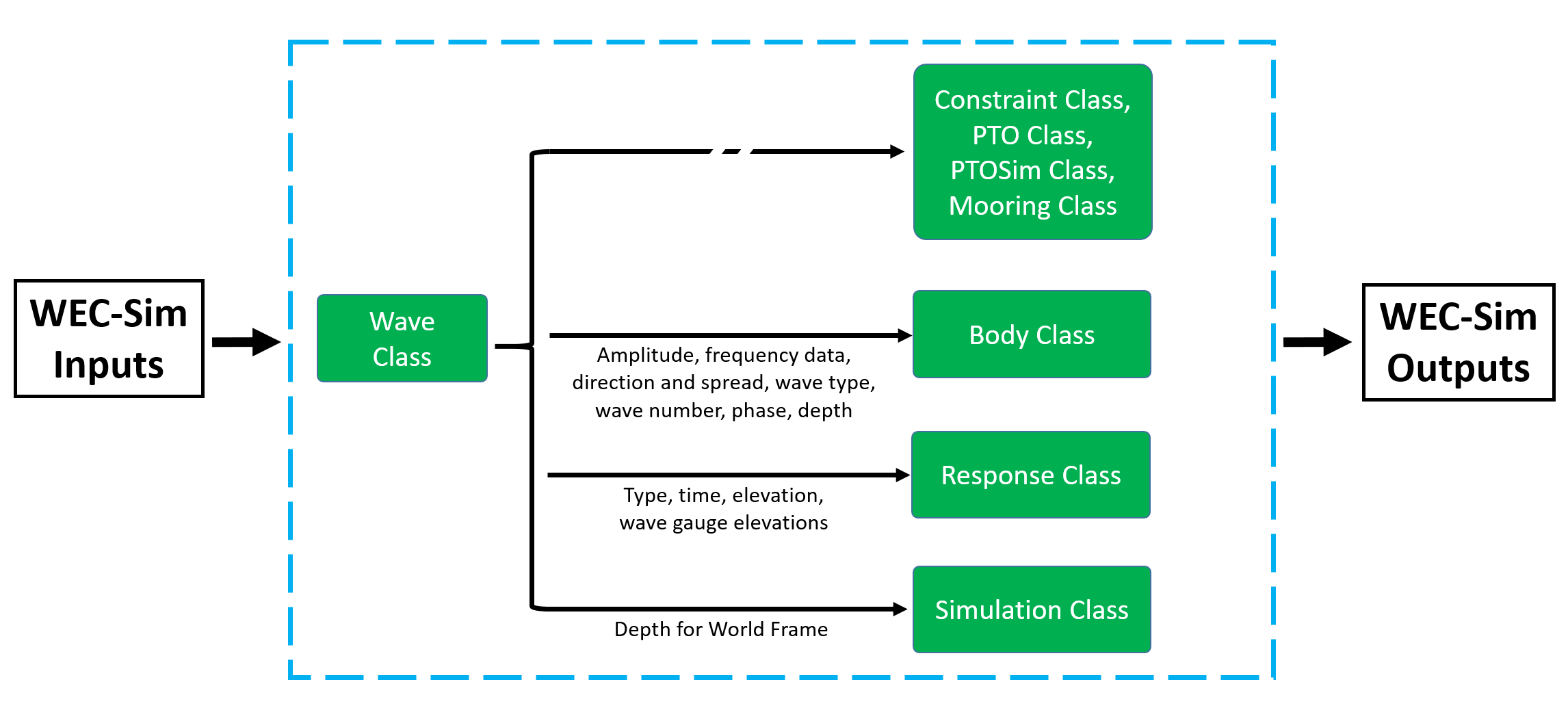
The wave class contains all wave information necessary to define the incident wave condition for the WEC-Sim time-domain simulation. The wave class contains the incoming wave information that determines the excitation force, added mass, radiation damping and other frequency based parameters that influence a body’s motion.
At a high level, the wave class interacts with the rest of WEC-Sim as shown in the diagram below. The wave primarily interacts with the body class through the pre-processing of wave forces and in Simulink.
Wave Class Initialization
Within the wecSimInputFile.m, users
must initialize the wave class (waveClass) and specify the waveType by
including the following line:
waves = waveClass('<waveType>');
Users must specify additional wave class properties using the waves object
depending on which wave type is selected, as shown in the table below. A more
detailed description of the available wave types is given in the following
sections.
Wave Type |
Required Properties |
|
|
|
|
|
|
|
|
|
|
|
|
|
|
|
|
Available wave class properties, default values, and functions can be found by
typing doc waveClass in the MATLAB command window, or by opening the
waveClass.m file in $WECSIM/source/objects directory by typing open
waveClass in the Matlab Command Window.
For more information about application of WEC-Sim’s wave class, refer to
Wave Features.
noWave
The noWave case is for running WEC-Sim simulations with no waves and
constant radiation added mass and wave damping coefficients. The noWave
case is typically used to run decay tests. Users must still provide hydro
coefficients from a BEM solver before executing WEC-Sim and specify the period
(wave.T) from which the hydrodynamic coefficients are selected.
The noWave case is defined by including the following in the input file:
waves = waveClass('noWave');
waves.period = <wavePeriod>; %[s]
noWaveCIC
The noWaveCIC case is the same as the noWave case described above, but with
the addition of the convolution integral calculation. The only difference is
that the radiation forces are calculated using the convolution integral and the
infinite frequency added mass.
The noWaveCIC case is defined by including the following in the input file:
waves = waveClass('noWaveCIC');
regular
The regular wave case is used for running simulations in regular waves with
constant radiation added mass and wave damping coefficients. Using this option,
WEC-Sim assumes that the system dynamic response is in sinusoidal steady-state
form, where constant added mass and damping coefficients are used (instead of
the convolution integral) to calculate wave radiation forces. Wave period
(wave.T) and wave height (wave.H) must be specified in the input file.
The regular case is defined by including the following in the input file:
waves = waveClass('regular');
waves.period = <wavePeriod>; %[s]
waves.height = <waveHeight>; %[m]
regularCIC
The regularCIC is the same as regular wave case described above, but with
the addition of the convolution integral calculation. The only difference is
that the radiation forces are calculated using the convolution integral and the
infinite frequency added mass. Wave period (wave.T) and wave height
(wave.H) must be specified in the input file.
The regularCIC case is defined by including the following in the input file:
waves = waveClass('regularCIC');
waves.period = <wavePeriod>; %[s]
waves.height = <waveHeight>; %[m]
irregular
The irregular wave case is the wave type for irregular wave simulations
using a Pierson Moskowitz (PM) or JONSWAP (JS) wave spectrum as defined by the
IEC TS 62600-2:2019 standards. Significant wave height (wave.H), peak
period (wave.T), and wave spectrum type (waves.spectrumtype) must be
specified in the input file. The available wave spectra and their corresponding
waves.spectrumType are listed below:
Wave Spectrum |
spectrumType |
Pierson Moskowitz |
|
JONSWAP |
|
The irregular case is defined by including the following in the input file:
waves = waveClass('irregular');
waves.period = <wavePeriod>; %[s]
waves.height = <waveHeight>; %[m]
waves.spectrumType = '<waveSpectrum>';
When using the JONSWAP spectrum, users have the option of defining gamma by
specifying waves.gamma = <waveGamma>;. If gamma is not defined,
then gamma is calculated based on a relationship between significant wave
height and peak period defined by IEC TS 62600-2:2019.
spectrumImport
The spectrumImport case is the wave type for irregular wave simulations
using an imported wave spectrum (ex: from buoy data). The user-defined spectrum
must be defined with the wave frequency (Hz) in the first column, and the
spectral energy density (m^2/Hz) in the second column. Users have the option to
specify a third column with phase (rad); if phase is not specified by the user
it will be randomly defined. An example file is provided in the
$WECSIM/examples/*/spectrumData.mat directory. The spectrumImport case is defined by including the following
in the input file:
waves = waveClass('spectrumImport');
waves.spectrumFile ='<spectrumFile >.mat';
Note
When using the spectrumImport or spectrumImportFullDir option, users must specify a sufficient
number of wave frequencies (typically ~1000) to adequately describe the
wave spectra. These wave frequencies are the same that will be used to
define the wave forces on the WEC, for more information refer to the
Irregular Wave Binning section.
spectrumImportFullDir
The spectrumImportFullDir case is for irregular wave simulations where the imported wave spectrum
is both frequency and directionally dependent. The user-defined spectrum file must contain a variable
called frequencies defining the wave frequencies (Hz), directions defining the wave directions
(degrees), spectrum defining the omni-directional wave spectrum (m^2/Hz), and spread defining the
frequency and directionally dependent wave spread (1/Hz/rad). The wave spread (in accordance
with the IEC TS 62600-2 standard) should satisfy:
\(\int_{-\pi}^{\pi} D(f, \theta) \, d\theta = 1\)
If specified, wave phase must be a rectangular matrix of size [i,j], where \(i\) is the number of wave frequencies and \(j\) is the number of directional bins. To generate a random spectra, specifying a single phase seed value (e.g., waves.phaseSeed = 128) is sufficient to ensure that the generated wave spectra is repeatable.
Note
At this time, the full directional wave spectra does NOT work with nonlinear hydrodynamics.
elevationImport
The elevationImport case is the wave type for wave simulations using user-defined
time-series (ex: from experiments). The user-defined wave surface elevation
must be defined with the time (s) in the first column, and the wave surface
elevation (m) in the second column. An example of this is given in the
elevationData.mat file in the tutorials directory folder of the WEC-Sim source
code. The elevationImport case is defined by including the following in the input
file:
waves = waveClass('elevationImport');
waves.elevationFile ='<elevationFile>.mat';
When using the elevationImport option, excitation forces are calculated via
convolution with the excitation impulse response function. This solution method
is not particularly robust and the quality of the results can depend heavily on
the discretization and range of the BEM data. This is especially true for elevation
data that contains a small number of frequencies (e.g., an approximation of regular
wave). Further, a number of advanced features are not available for this solution
method. Direct multiplication of the frequency components, as performed in the
spectrumImport and irregular methods is a more robust and capable approach,
but requires developing a ‘<spectrumFile>.mat’ that is time-domain equivalent to ‘<elevationFile>.mat’.
For this workflow, the elevationToSpectrum function has been provided in
$WEC-Sim/source/functions/BEMIO.
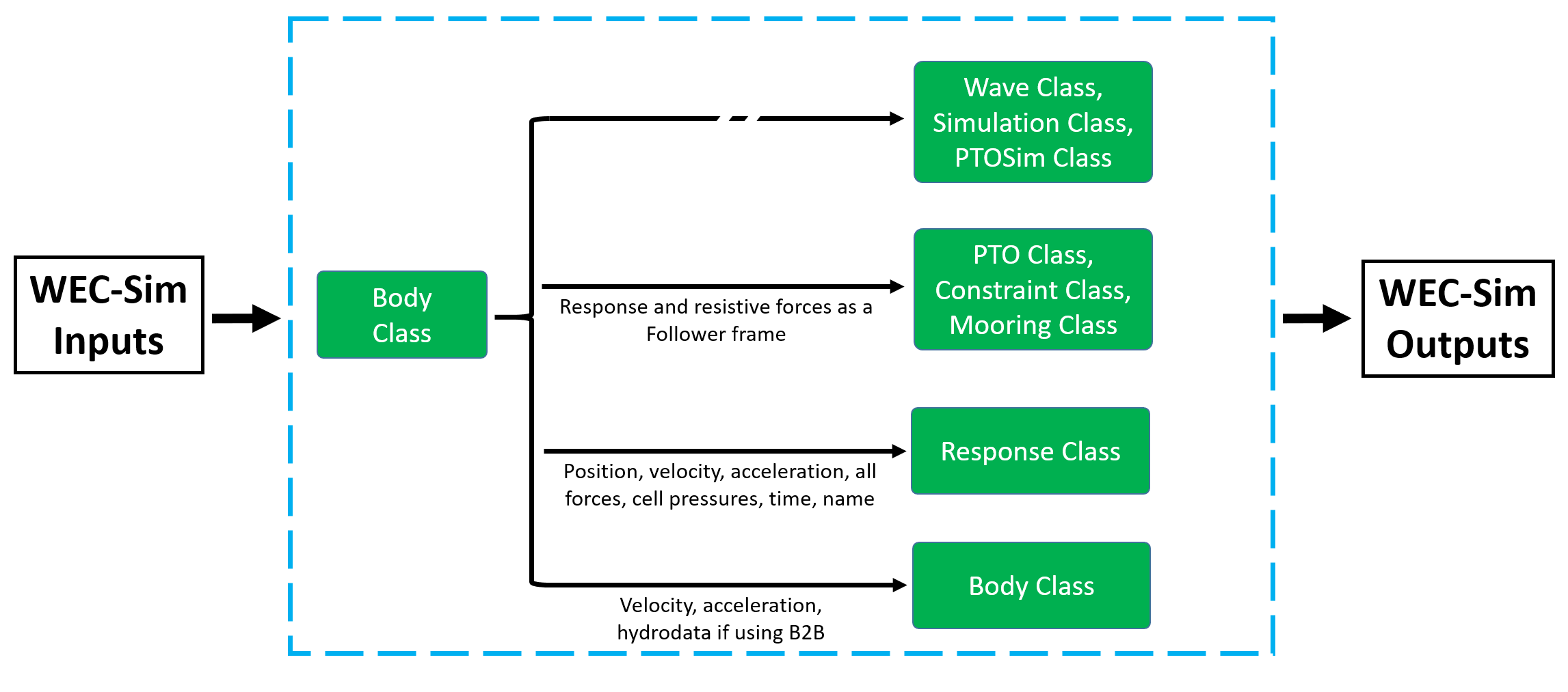
Body Class
The body class represents each rigid or flexible body that comprises the WEC
being simulated. It contains the mass and hydrodynamic properties of each body,
defined by hydrodynamic data from the *.h5 file. The corresponding body block
uses the hydrodynamic data and wave class to calculate all relevant forces on
the body and solve for its resultant motion. At a high level, the body class
interacts with the rest of WEC-Sim as shown in the diagram below.
Bodies hold hydrodynamic BEM input data, calculate body forces and pass forces
and motions to other Simulink blocks.
Body Class Initialization
Within the wecSimInputFile.m,
users must initialize each iteration of the body class (bodyClass), and
specify the location of the hydrodynamic data file (<bemData>.h5) and geometry
file (<geomFile>.stl) for each body. The body class is defined by including the
following lines in the WEC-Sim input file, where i is the body number and
‘<bem_data>.h5’ is the name of the h5 file containing the BEM results:
body(i)=bodyClass('<bemData>.h5')
body(i).geometryFile = '<geomFile>.stl';
WEC-Sim bodies may be one of three types: hydrodynamic, drag, or flexible. These types represent varying degrees of complexity and require various input parameters and BEM data, detailed in the table below. The Body Features section contains more details on these important distinctions.
Body Type |
Description |
|---|---|
Hydrodynamic Body |
|
Drag Body |
|
Flexible Body |
|
Users may specify other body class properties using the body object for
each body in the wecSimInputFile.m.
Important body class properties include quantities such as
the mass, moment of inertia, center of gravity and center of buoyancy.
Other parameters are specified as needed.
For example, viscous drag can be specified by entering the viscous drag
coefficient and the characteristic area in vector format the WEC-Sim
input file as follows:
body(i).quadDrag.cd = [0 0 1.3 0 0 0]
body(i).quadDrag.area = [0 0 100 0 0 0]
Available body properties, default values, and functions can be found by typing
doc bodyClass in the MATLAB command window, or opening the bodyClass.m
file in $WECSIM/source/objects directory by typing open bodyClass in
Matlab Command Window.
For more information about application of WEC-Sim’s body class, refer to
Body Features.
Note
The *.h5 file defines the hydrodynamic data for all relevant bodies. It is
required that any drag body or nonhydrodyamic body be numbered after all
hydrodynamic bodies The body index must correspond with the index in the
*.h5 file and the number in the Simulink diagram.
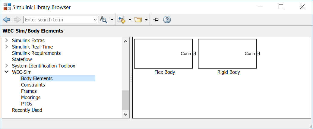
Body Blocks
The Body Elements library shown below contains two blocks:
the Rigid Body block and the Flex Body block. The rigid body block is
used to represent hydrodynamic and drag bodies, each subset being
a Variant Sub-system of a Rigid Body.
Before simulation, one variant is activated by a flag in the body object
(body.nonHydro=0,1,2). The flex body block is used to represent hydrodynamic
bodies that contain additional flexible degrees of freedom (‘generalized body
modes’). The flex body is determined automatically by the degrees of freedom
contained in the BEM input data. At least one instance of a body
block (rigid or flex) is required in each model. The
Body Features section describes the various types of
WEC-Sim bodies in detail.
Both in Simulink and the input file, the user has to name the blocks
body(i) (where i=1,2,…). The mass properties, hydrodynamic data, geometry
file, mooring, and other properties are then specified in the input file.
Within the body block, the wave radiation, wave excitation, hydrostatic
restoring, viscous damping, and mooring forces are calculated.
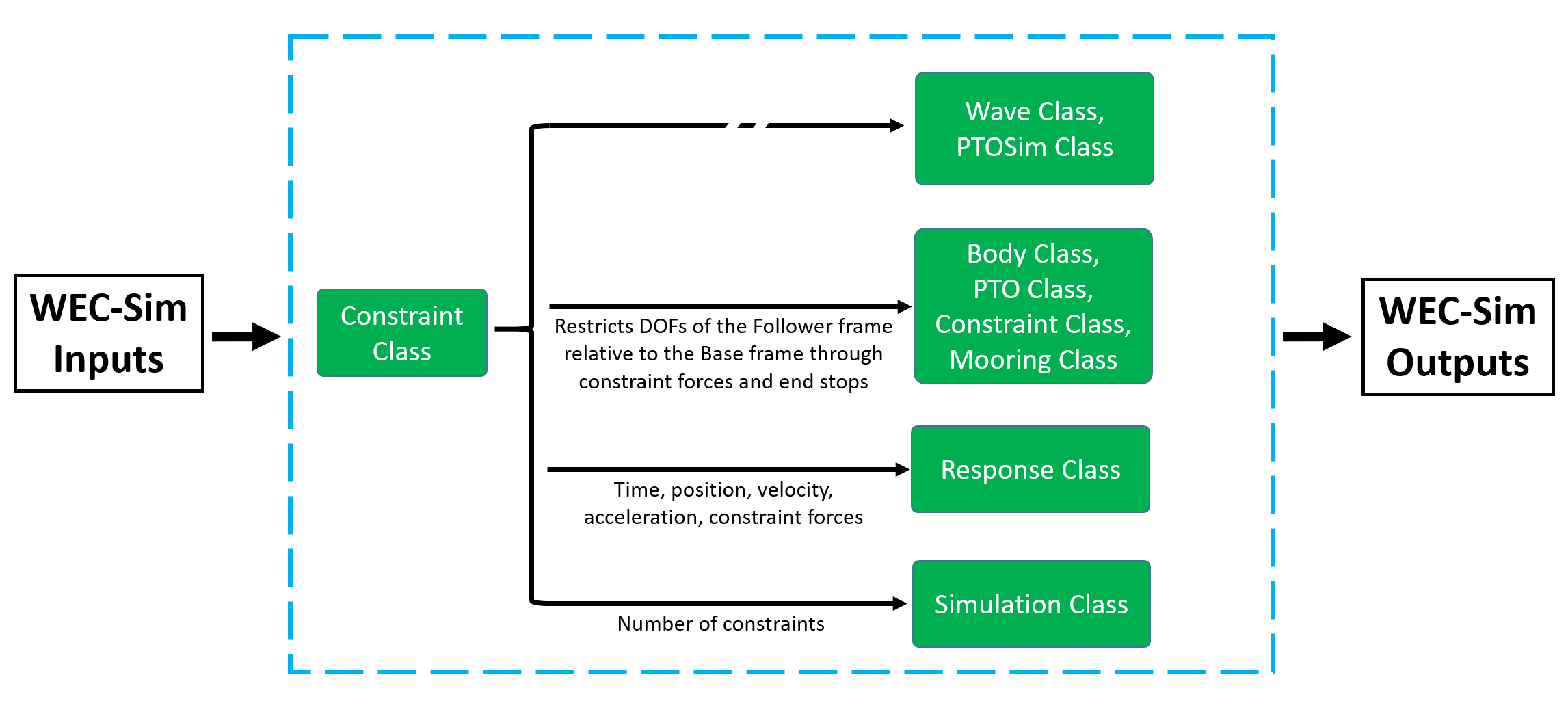
Constraint Class
The WEC-Sim constraint class and blocks connect WEC bodies to one another (and possibly to the seabed) by constraining DOFs. Constraint objects do not apply any force or resistance to body motion outside of the reactive force required to prevent motion in a given DOF. At a high level, the constraint class interacts with the rest of WEC-Sim as shown in the diagram below. Constraint objects largely interact with other blocks through Simscape connections that pass resistive forces to other bodies, constraints, ptos, etc.
Constraint Class Initialization
The properties of the constraint class (constraintClass) are defined in the
constraint object. Within the wecSimInputFile.m, users must initialize
each iteration the constraint class (constraintClass) and specify the
constraintName, by including the following lines:
constraint(i)=constraintClass('<constraintName>');
For rotational constraint (ex: pitch), users may also specify the location and orientation of the rotational joint with respect to the global reference frame:
constraint(i).location = [<x> <y> <z>];
constraint(i).orientation.z = [<x> <y> <z>];
constraint(i).orientation.y = [<x> <y> <z>];
Available constraint properties, default values, and functions can be found by
typing doc constraintClass in the MATLAB command window, or opening the
constraintClass.m file in $WECSIM/source/objects directory by typing
open constraintClass in MATLAB Command Window.
For more information about application of WEC-Sim’s constraint class, refer to
Constraint and PTO Features.
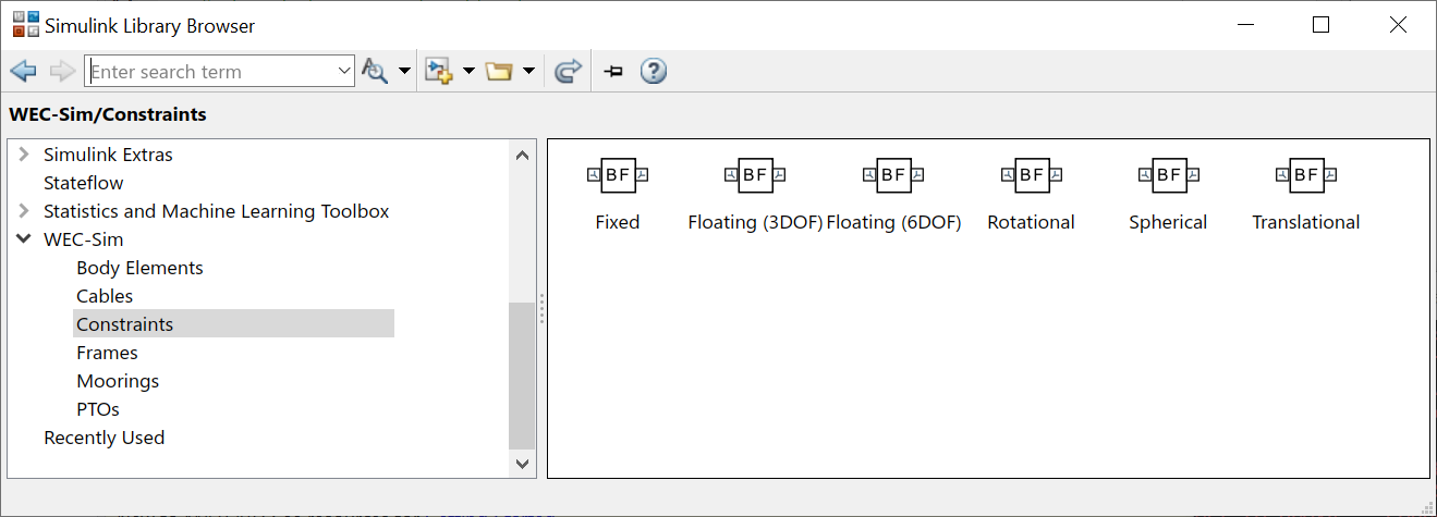
Constraint Blocks
The Constraint Class is tied to the blocks within the Constraints library.
These are used to define the DOF of a
specific body. Constraint blocks define only the DOF, but do not otherwise
apply any forcing or resistance to the body motion. Each Constraint block has
two connections: a base (B) and a follower (F). The Constraints block restricts
the motion of the block that is connected to the follower relative to the block
that is connected to the base. For a single body system, the base would be the
Global Reference Frame and the follower is a Rigid Body.
A brief description of each constraint block is given below. More information can also be found by double clicking on the library block and viewing the Block Parameters box.
Constraint Library |
||
|---|---|---|
Block |
DOFs |
Description |
|
0 |
Rigid connection. Constrains all motion between the base and follower |
|
1 |
Constrains the motion of the follower relative to the base to be translation along the constraint’s Z-axis |
|
1 |
Constrains the motion of the follower relative to the base to be rotation about the constraint’s Y-axis |
|
3 |
Contrains the motion of the follower relative to the base to be rotation about the X-, Y-, and Z- axis. |
|
3 |
Constrains the motion of the follower relative to the base to planar motion with translation along the constraint’s X- and Z- and rotation about the Y- axis |
|
6 |
Allows for unconstrained motion of the follower relative to the base |
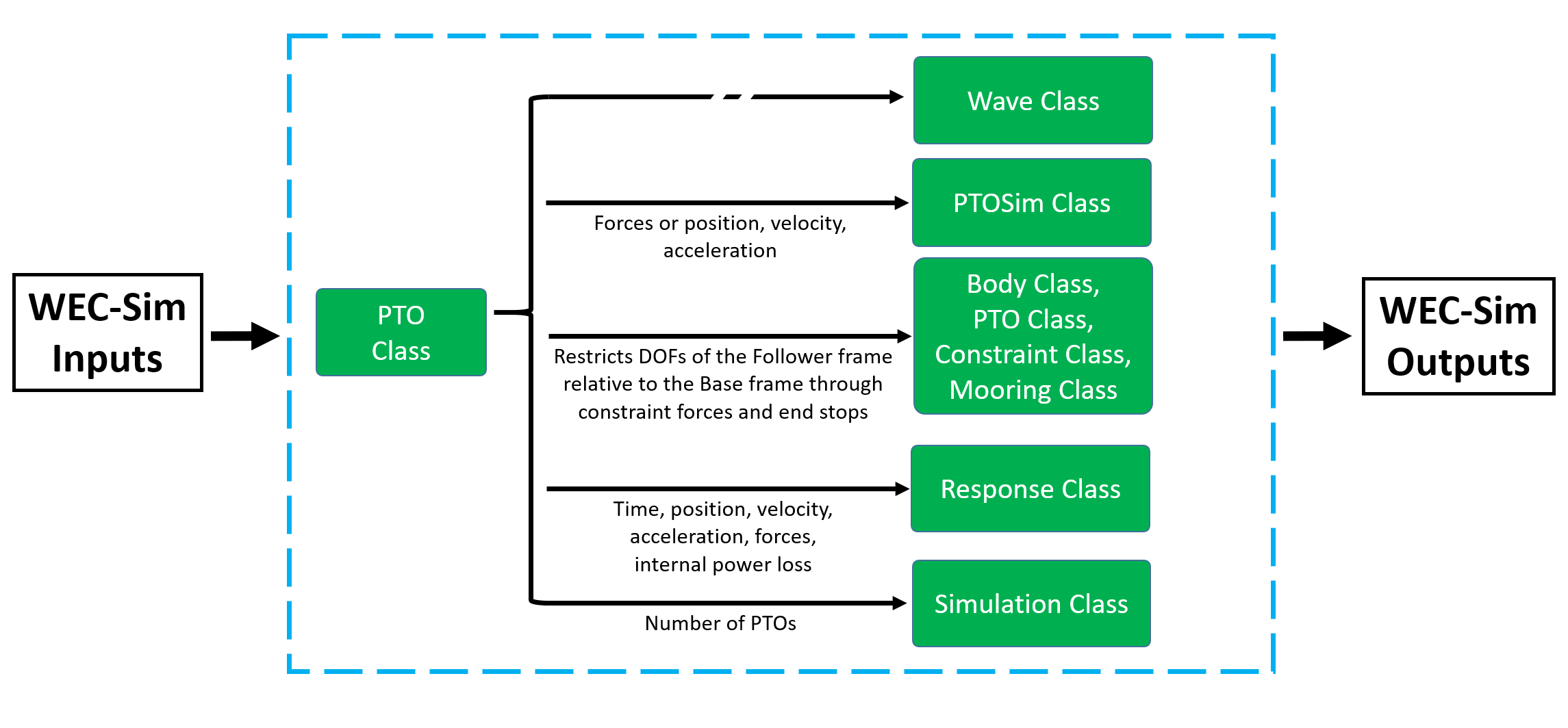
PTO Class
WEC-Sim Power Take-Off (PTO) blocks connect WEC bodies to one other (and possibly to the seabed) by constraining DOFs and applying linear damping and stiffness. The ability to apply damping, stiffness, or other external forcing differentiates a ‘PTO’ from a ‘Constraint’. The damping and stiffness allow a pto to extract power from relative body motion with respect to a fixed reference frame or another body.
At a high level, the PTO class interacts with the rest of WEC-Sim as shown in the diagram below. PTO objects largely interact with other blocks through Simscape connections that pass resistive forces to other bodies, constraints, ptos, etc.
PTO Class Initialization
The properties of the PTO class (ptoClass) are
defined in the pto object. Within the wecSimInputFile.m, users must
initialize each iteration the pto class (ptoClass) and specify the
ptoName, by including the following lines:
pto(i) = ptoClass('<ptoName>');
For rotational ptos, the user also needs to specify the location of the
rotational joint with respect to the global reference frame in the
pto(i).location variable. In the PTO class, users can also specify
linear damping (pto(i).damping) and stiffness (pto(i).stiffness) values to
represent the PTO system (both have a default value of 0). Users can overwrite
the default values in the input file. For example, users can specify a damping
value by entering the following in the WEC-Sim input file:
pto(i).damping = <ptoDamping>;
pto(i).stiffness = <ptoStiffness>;
Available pto properties, default values, and functions can be found by typing
doc ptoClass in the MATLAB command window, or opening the ptoClass.m file
in $WECSIM/source/objects directory by typing open ptoClass in MATLAB
Command Window.
For more information about application of WEC-Sim’s pto class, refer to
Constraint and PTO Features.
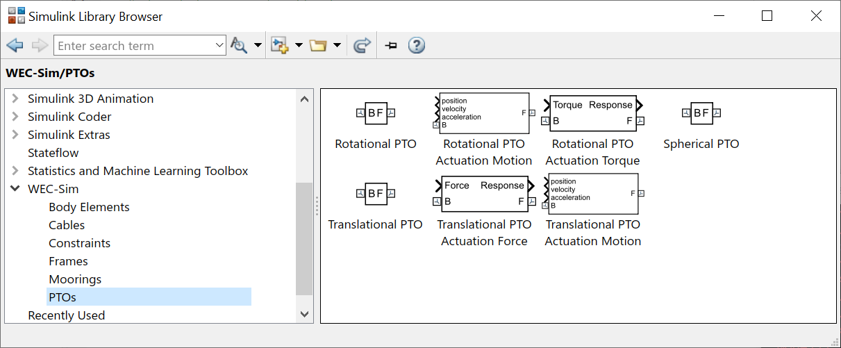
PTO Blocks
The PTO Class is tied to the PTOs library.
Similar to the Constraint blocks, the PTO blocks have a base (B) and
a follower (F). Users must name each PTO block pto(i)
(where i=1,2,…) and then define their properties in the input file.
The Translational PTO, Spherical PTO, and Rotational PTO are identical to the
Translational, Spherical, and Rotational constraints, but they allow for the
application of linear damping and stiffness forces. Additionally, there are two
other variations of the Translational and Rotational PTOs. The Actuation
Force/Torque PTOs allow the user to define the PTO force/torque at each
time-step and provide the position, velocity and acceleration of the PTO at
each time-step. The user can use the response information to calculate the PTO
force/torque. The Actuation Motion PTOs allow the user to define the motion of
the PTO. These can be useful to simulate forced-oscillation tests.
Note
When using the Actuation Force/Torque PTO or Actuation Motion PTO blocks, the loads and displacements are specified in the local (not global) coordinate system. This is true for both the sensed (measured) and actuated (commanded) loads and displacements.
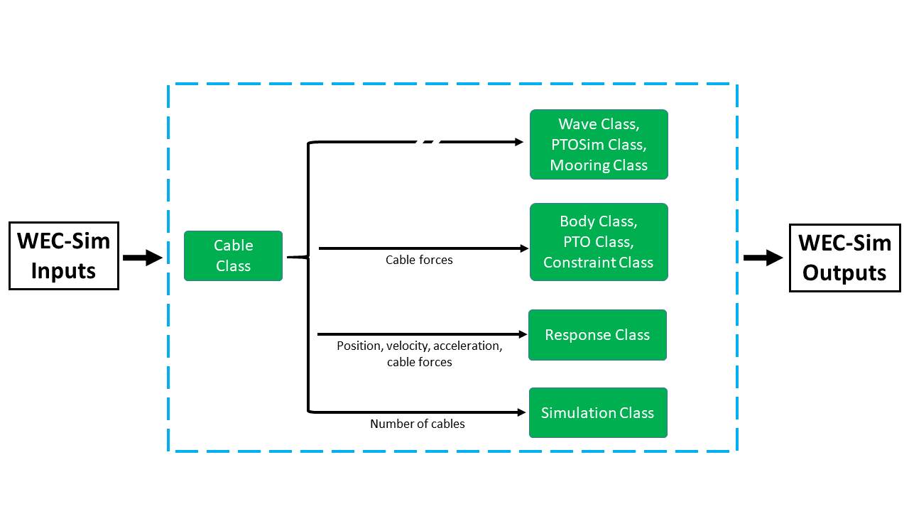
Cable Class
WEC-Sim Cable blocks connect WEC bodies to one other by a cable. They allows users to apply damping and/or stiffness when the cable is in tension, but allow no forcing in compression. At a high level, the cable class interacts with the rest of WEC-Sim as shown in the diagram below.
Cable Class Initialization
The properties of the cable class (cableClass) are defined in the cable object.
Within the wecSimInputFile.m, users must initialize the cable class and specify the
cableName, in addition to the baseConnection and followerConnection (in that order), by including the following lines:
cable(i) = cableClass('cableName','baseConnection','followerConnection');
cable(i).damping = <cableDamping>;
cable(i).stiffness = <cableStiffness>;
Available cable properties, default values, and functions
can be found by typing doc cableClass in the MATLAB command window, or
opening the cableClass.m file in $WECSIM/source/objects directory by
typing open cableClass in MATLAB Command Window.
For more information about application of WEC-Sim’s mooring class, refer to
Cable Features.
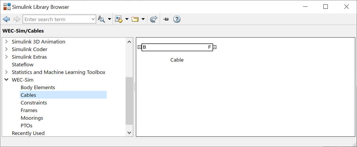
Cable Block
The Cable Class is tied to the Cables library.
The Cable block applies linear damping and stiffness based on
the motion between the base and follower.
Cables can be used between two bodies to apply a coupling force only when taut or stretched.
A cable block must be added to the model between two PTOs or constraints that are to be connected by the cable.
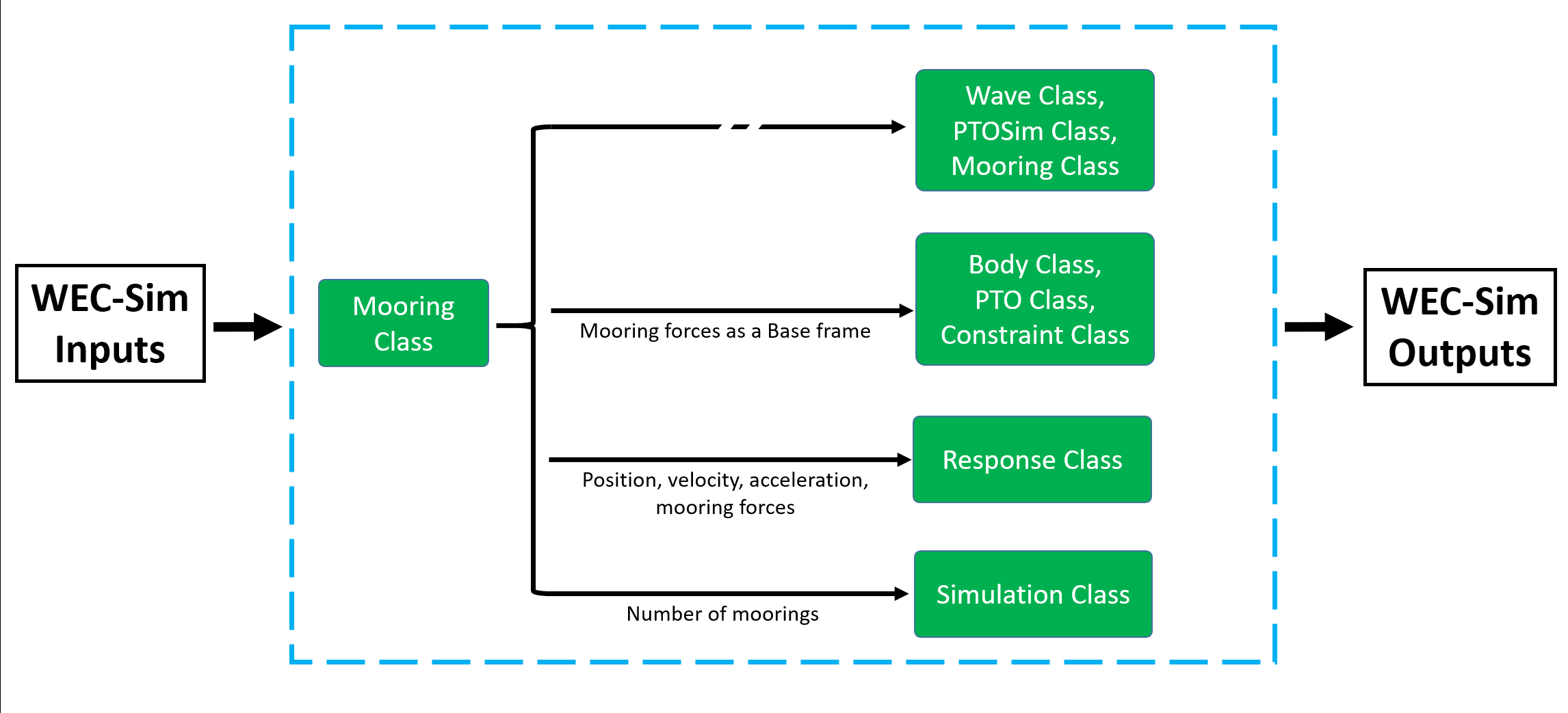
Mooring Class
The mooring class (mooringClass) allows for different fidelity simulations
of mooring systems. Three possibilities are available, a lumped mooring matrix,
a mooring lookup table, or MoorDyn. These differences are determined by the Simulink block(s) chosen, and are
described below. At a high level, the Mooring class interacts with the rest of
WEC-Sim as shown in the diagram below. The interaction is similar to a
constraint or PTO, where some resistive forcing is calculated and passed to a
body block through a Simscape connection.
Mooring Class Initialization
The properties of the mooring class (mooringClass) are defined in the
mooring object. Within the wecSimInputFile.m, users must initialize
the mooring class and specify the mooringName, by including the following lines:
mooring(i)= mooringClass('<mooringName>');
Available mooring properties, default values, and functions
can be found by typing doc mooringClass in the MATLAB command window, or
opening the mooringClass.m file in $WECSIM/source/objects directory by
typing open mooringClass in MATLAB Command Window.
For more information about application of WEC-Sim’s mooring class, refer to
Mooring Features.
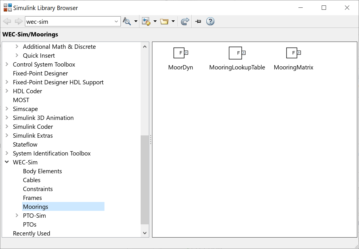
Mooring Blocks
The Mooring Class is tied to the Moorings library.
Four types of blocks may be used: a ‘Mooring Matrix’, a ‘Mooring Lookup Table’,
a ‘MoorDyn Connection’ block, or a ‘MoorDyn Caller’ block.
The MooringMatrix block applies linear damping and stiffness based on
the motion of the follower relative to the base.
Damping and stiffness can be specified between all DOFs in a 6x6 matrix.
The MooringLookupTable block searches a user-supplied 6DOF force lookup table.
The lookup table should contain six parameters: the resultant mooring force in each degree of freedom.
Each force is indexed by position in all six degrees of freedom.
The mooring force is interpolated between indexed positions based on the instantaneous position of the mooring system.
There are no restrictions on the number of MooringMatrix or MooringLookupTable blocks.
The MoorDynConnection block is used to detect the relative motion between
two connection points (i.e., a body and the global reference frame or between
two bodies). The block uses Simulink’s ‘Goto’ and ‘From’ blocks to feed the
relative response to the MoorDynCaller block, which then calls MoorDyn to
calculate the 6 degree of freedom mooring forces based on the instantaneous displacement,
velocity, a MoorDyn input file, and the compiled MoorDyn libraries to simulate a realistic
mooring system. The mooring forces are then sent back to the MoorDyn Connection
block to be applied at the body’s center of gravity. Multiple MoorDyn Connection
blocks can be used to specify mooring lines between different bodies/frames,
but there can only be one MoorDyn Caller block per Simulink model. Each
MoorDyn Connection block should be initialized as a mooring object in
the wecSimInputFile.m with mooring(i).moorDyn set equal to 1. The
MoorDynCaller block should not have an accompanying mooring object.
If set up correctly in the wecSimInputFile.m, the signals will be
automatically sent between the MoorDyn Connection and MoorDyn Caller blocks.
PTO-Sim Class
The PTO-Sim class contains all the information for the PTO-Sim blocks, which can be used to simulate PTO systems. The difference beetween the PTO-Sim class and the PTO class is that the PTO-Sim class have detailed models of different components that are used in PTO systems such as hydraulic cylinders, hydraulic accumulators, hydraulic motors, electric generators, etc., while the PTO class have a linear parametric model that summarizes the PTO dynamics with a stiffness and a damping term. At a high level, the PTO-Sim class interacts with the rest of WEC-Sim as shown in the diagram below:
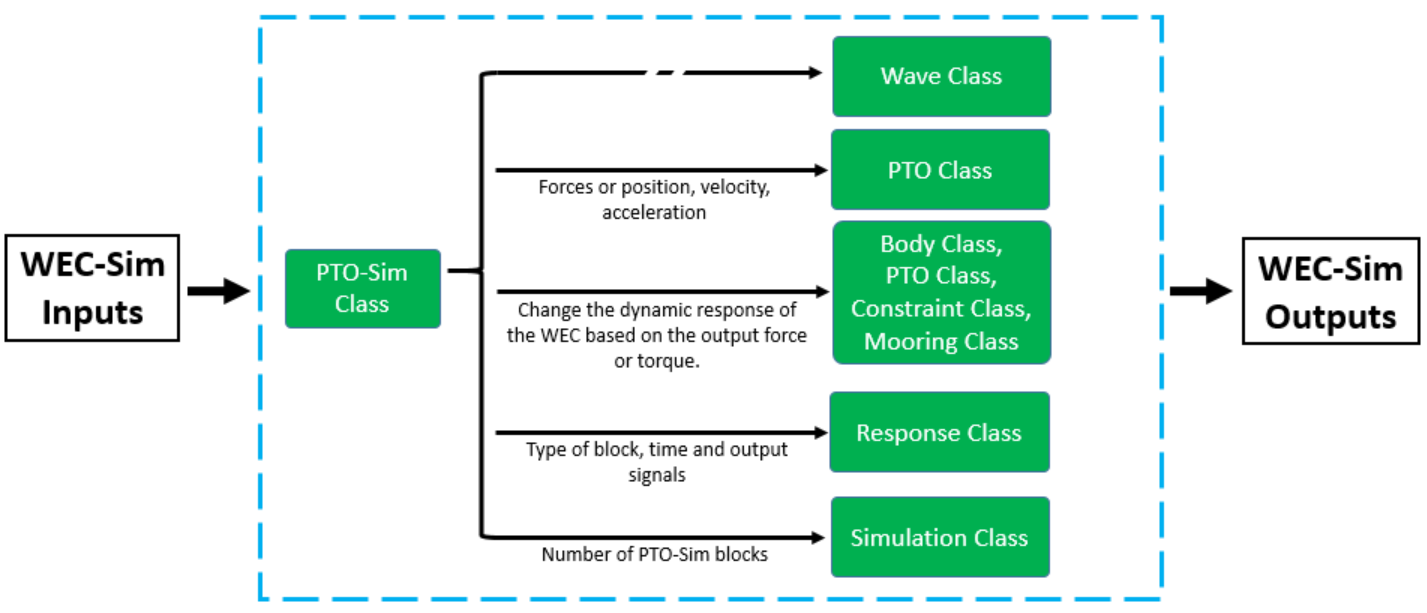
The PTO-Sim blocks receive the linear or angular response from the PTO blocks and give either the torque or the force depending on the PTO dynamics.
PTO-Sim Class Initialization
The properties of the PTO-Sim class (ptoSimClass) are defined in the ptoSim object. The PTO-Sim class must be
initialized in the wecSimInputFile.m script. There are three properties that must be initialized for all the PTO-Sim blocks,
those are the name, the block number, and the type:
ptoSim(i) = ptoSimClass('ptoSimName');
ptoSim(i).ptoSimNum = i;
ptoSim(i).ptoSimType = <TypeNumber>;
The type value must be defined depending on the type of block used in the simulation as follows:
PTO-Sim Library |
|
|---|---|
Block |
Type |
Electric Generator |
1 |
Hydraulic cylinder |
2 |
Hydraulic accumulator |
3 |
Rectifying check valve |
4 |
Hydraulic motor |
5 |
Linear crank |
6 |
Adjustable rod |
7 |
Check valve |
8 |
Direct drive linear generator |
9 |
Direct drive rotary generator |
10 |
Available PTO-Sim blocks properties, default values, and functions
can be found by typing doc ptoSimClass in the MATLAB command window, or
opening the ptoSimClass.m file in $WECSIM/source/objects directory by
typing open ptoSimClass in MATLAB Command Window.
For more information about application of WEC-Sim’s mooring class, refer to
Constraint and PTO Features.
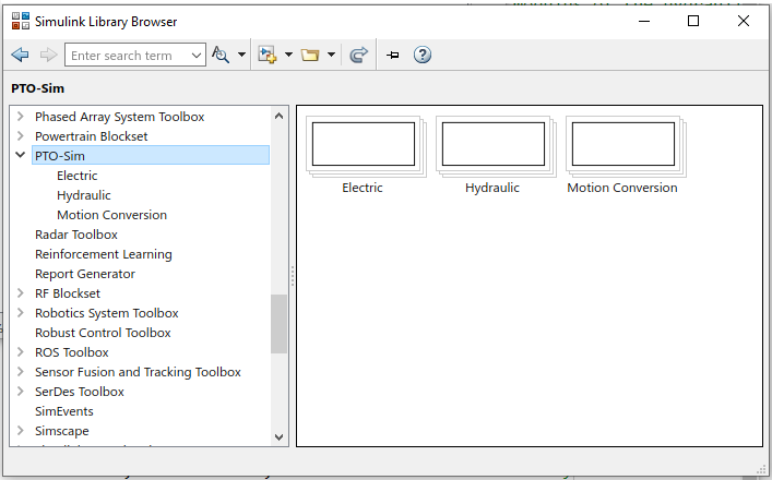
PTO-Sim Blocks
There are eight different types of blocks in the PTO-Sim class divided in three sub-categories: Hydraulic, Electric, and Motion Conversion. In the hydraulic sub-category there are five blocks: Check Valve, Compressible Fluid Piston, Gas-Charged Hydraulic Accumulator, Hydraulic Motor, and Rectifying Check Valve. In the Electric sub-category there is a block call Electric Generator Equivalent Circuit which models an electric generator with an equivalent circuit. The motion conversion blocks (Rotary to Linear Adjustable Rod, and Rotary to Linear Crank) can be used to to convert rotational motion into linear motion to add a hydraulic cylinder to the PTO model. There are no restrictions on the number of PTO-Sim blocks.
Response Class
The response class contains all the output time-series and methods to plot and interact with the results. It is not initialized by the user, and there is no related Simulink block. Instead, it is created automatically at the end of a WEC-Sim simulation. The response class does not input any parameter back to WEC-Sim, only taking output data from the various objects and blocks.
After WEC-Sim is done running, there will be a new variable called output
saved to the MATLAB workspace. The output object is an instance of the
responseClass. It contains all the relevant time-series results of the
simulation. Time-series are given as [# of time-steps x 6] arrays, where 6 is the degrees of freedom.
Refer to the WEC-Sim API documentation for the Response Class for
information about the structure of the output object, .
Functions & External Codes
While the bulk of the WEC-Sim code consists of the WEC-Sim classes and the
WEC-Sim library, the source code also includes supporting functions and
external codes. These include third party Matlab functions to read *.h5 and
*.stl files, WEC-Sim Matlab functions to write *.h5 files and run
WEC-Sim in batch mode, MoorDyn compiled libraries, python macros for ParaView
visualization, and the PTO-Sim class and library. Additionally, BEMIO can be
used to create the hydrodynamic *.h5 file required by WEC-Sim. MoorDyn is
an open source code that must be downloaded separately. Users may also obtain,
modify, and recompile the code as desired.
External Simulink/Simscape Blocks
In some situations, users may want to use Simulink/Simscape blocks that are not included in the WEC-Sim Library to build their WEC model. External blocks may be linked to the standard WEC-Sim library to implement controllers, additional bodies, complex power take-offs and other custom designs.
Note
The Simulink Mechanism Configuration for automatic gravity calculations is not used in WEC-Sim. Gravity is instead defined as a force that is combined with the buoyancy force. Users who wish to add external bodies should account for gravity by:
Create nonhydrodynamic bodies with zero displaced volume, or
Manually add the gravity force into their external functionality